开始之前
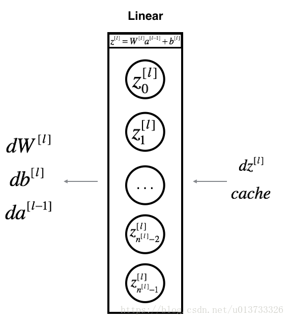
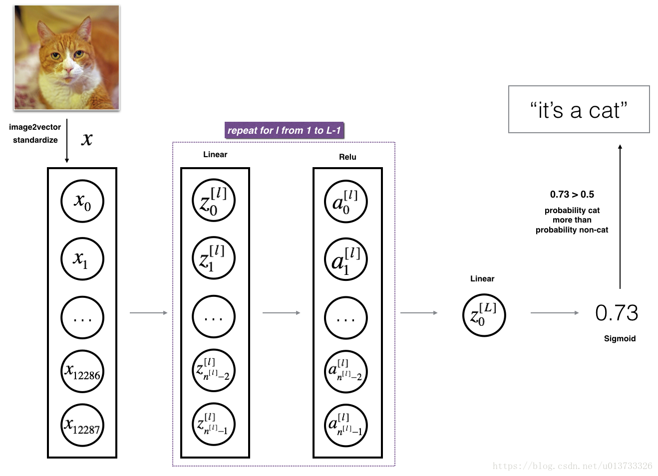
在正式开始之前,我们先来了解一下我们要做什么。在本次教程中,我们要构建两个神经网络,一个是构建两层的神经网络,一个是构建多层的神经网络,多层神经网络的层数可以自己定义。本次的教程的难度有所提升,但是我会力求深入简出。在这里,我们简单的讲一下难点,本文会提到**[LINEAR-> ACTIVATION]转发函数,比如我有一个多层的神经网络,结构是输入层->隐藏层->隐藏层->・・・->隐藏层->输出层**,在每一层中,我会首先计算Z = np.dot(W,A) + b,这叫做【linear_forward】,然后再计算A = relu(Z) 或者 A = sigmoid(Z),这叫做【linear_activation_forward】,合并起来就是这一层的计算方法,所以每一层的计算都有两个步骤,先是计算Z,再计算A,你也可以参照下图:
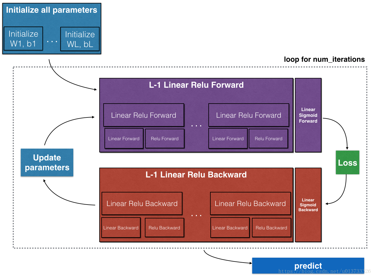
我们来说一下步骤:
1.初始化网络参数
2.前向传播
2.1 计算一层的中线性求和的部分
2.2 计算激活函数的部分(ReLU使用L-1次,Sigmod使用1次)
2.3 结合线性求和与激活函数
3.计算误差
4.反向传播
4.1 线性部分的反向传播公式
4.2 激活函数部分的反向传播公式
4.3 结合线性部分与激活函数的反向传播公式
5.更新参数
请注意,对于每个前向函数,都有一个相应的后向函数。 这就是为什么在我们的转发模块的每一步都会在cache中存储一些值,cache的值对计算梯度很有用, 在反向传播模块中,我们将使用cache来计算梯度。 现在我们正式开始分别构建两层神经网络和多层神经网络。
准备软件包
在开始我们需要准备一些软件包:
import numpy as np
import h5py
import matplotlib.pyplot as plt
import testCases #参见资料包,或者在文章底部copy
from dnn_utils import sigmoid, sigmoid_backward, relu, relu_backward #参见资料包
import lr_utils #参见资料包,或者在文章底部copy# 指定随机种子
np.random.seed(1)
初始化参数
对于一个两层的神经网络结构而言,模型结构是线性->ReLU->线性->sigmod函数。
def initialize_parameters(n_x, n_h, n_y):'''此函数是为了初始化两层网络参数而使用的函数。参数:n_x - 输入层节点数量n_h - 隐藏层节点数量n_y - 输出层节点数量返回:parameters - 包含你的参数的python字典:W1 - 权重矩阵,维度为(n_h,n_x)b1 - 偏向量,维度为(n_h,1)W2 - 权重矩阵,维度为(n_y,n_h)b2 - 偏向量,维度为(n_y,1)'''# 乘以0.01是防止梯度下降缓慢W1 = np.random.randn(n_h, n_x) * 0.01b1 = np.zeros((n_h, 1))W2 = np.random.randn(n_y, n_h) * 0.01b2 = np.zeros((n_y, 1))# 使用断言来确保我的数据格式是正确的assert(W1.shape == (n_h ,n_x))assert(b1.shape == (n_h, 1))assert(W2.shape == (n_y, n_h))assert(b2.shape == (n_y, 1))parameters = {
    "W1": W1,"b1": b1,"W2": W2,"b2": b2}return parameters
初始化完成我们来测试一下:
print("==============测试initialize_parameters==============")
parameters = initialize_parameters(3,2,1)
print("W1 = " + str(parameters["W1"]))
print("b1 = " + str(parameters["b1"]))
print("W2 = " + str(parameters["W2"]))
print("b2 = " + str(parameters["b2"]))
==============测试initialize_parameters==============
W1 = [[ 0.01624345 -0.00611756 -0.00528172][-0.01072969  0.00865408 -0.02301539]]
b1 = [[0.][0.]]
W2 = [[ 0.01744812 -0.00761207]]
b2 = [[0.]]
L层的神经网络的初始化
def initialize_parameters_deep(layers_dims):'''此函数是为了初始化多层网络参数而使用的函数。参数:layers_dims - 包含我们网络中每个图层的节点数量的列表返回:parameters - 包含参数“W1”,“b1”,...,“WL”,“bL”的字典:W1 - 权重矩阵,维度为(layers_dims [1],layers_dims [1-1])bl - 偏向量,维度为(layers_dims [1],1)'''# 设置随机种子,来控制结果稳定np.random.seed(3)parameters = {
    }  #承载参数L = len(layers_dims)  #确定隐藏层层数# 隐藏层层数比传入的参数少一,不包括输入层和输出层# 随机初始化参数for l in range(1, L):parameters['W'+str(l)] = np.random.randn(layers_dims[l], layers_dims[l-1]) / np.sqrt(layers_dims[l-1])parameters['b'+str(l)] = np.zeros((layers_dims[l], 1))# 确保数据格式正确assert(parameters['W'+str(l)].shape == (layers_dims[l], layers_dims[l-1]))assert(parameters['b'+str(l)].shape == (layers_dims[l], 1))return parameters
测试一下:
#测试initialize_parameters_deep
print("==============测试initialize_parameters_deep==============")
layers_dims = [5,4,3]
parameters = initialize_parameters_deep(layers_dims)
print("W1 = " + str(parameters["W1"]))
print("b1 = " + str(parameters["b1"]))
print("W2 = " + str(parameters["W2"]))
print("b2 = " + str(parameters["b2"]))
==============测试initialize_parameters_deep==============
W1 = [[ 0.79989897  0.19521314  0.04315498 -0.83337927 -0.12405178][-0.15865304 -0.03700312 -0.28040323 -0.01959608 -0.21341839][-0.58757818  0.39561516  0.39413741  0.76454432  0.02237573][-0.18097724 -0.24389238 -0.69160568  0.43932807 -0.49241241]]
b1 = [[0.][0.][0.][0.]]
W2 = [[-0.59252326 -0.10282495  0.74307418  0.11835813][-0.51189257 -0.3564966   0.31262248 -0.08025668][-0.38441818 -0.11501536  0.37252813  0.98805539]]
b2 = [[0.][0.][0.]]
我们分别构建了两层和多层神经网络的初始化参数的函数,现在我们开始构建前向传播函数。
前向传播函数
前向传播有以下三个步骤
- LINEAR
- LINEAR - >ACTIVATION,其中激活函数将会使用ReLU或Sigmoid。
- [LINEAR - > RELU] ×(L-1) - > LINEAR - > SIGMOID(整个模型)
线性部分【LINEAR】
前向传播中,线性部分计算如下:
def linear_forward(A, W, b):'''实现前向传播的线性部分。参数:A - 来自上一层(或输入数据)的激活,维度为(上一层的节点数量,示例的数量)W - 权重矩阵,numpy数组,维度为(当前图层的节点数量,前一图层的节点数量)b - 偏向量,numpy向量,维度为(当前图层节点数量,1)返回:Z - 激活功能的输入,也称为预激活参数cache - 一个包含“A”,“W”和“b”的字典,存储这些变量以有效地计算后向传递'''Z = np.dot(W, A) + b #计算输入# 确保数据格式正确assert(Z.shape == (W.shape[0], A.shape[1]))cache = (A, W, b)return Z, cache
测试一下线性部分:
#测试linear_forward
print("==============测试linear_forward==============")
A,W,b = testCases.linear_forward_test_case()
Z,linear_cache = linear_forward(A,W,b)
print("Z = " + str(Z))
==============测试linear_forward==============
Z = [[ 3.26295337 -1.23429987]]
线性激活部分【LINEAR - >ACTIVATION】
为了更方便,我们将把两个功能(线性和激活)分组为一个功能(LINEAR-> ACTIVATION)。 因此,我们将实现一个执行LINEAR前进步骤,然后执行ACTIVATION前进步骤的功能。
A[l] = g(Z[l])
其中g是激活函数,sigmoid或者relu
def linear_activation_forward(A_prev, W, b, activation):'''实现LINEAR-> ACTIVATION 这一层的前向传播参数:A_prev - 来自上一层(或输入层)的激活,维度为(上一层的节点数量,示例数)W - 权重矩阵,numpy数组,维度为(当前层的节点数量,前一层的大小)b - 偏向量,numpy阵列,维度为(当前层的节点数量,1)activation - 选择在此层中使用的激活函数名,字符串类型,【"sigmoid" | "relu"】返回:A - 激活函数的输出,也称为激活后的值cache - 一个包含“linear_cache”和“activation_cache”的字典,我们需要存储它以有效地计算后向传递'''# 区分不同的激活函数if activation == 'sigmoid':# 前向传播Z, linear_cache = linear_forward(A_prev, W, b)A, activation_cache = sigmoid(Z)elif activation == 'relu':Z, linear_cache = linear_forward(A_prev, W, b)A, activation_cache = relu(Z)#确保数据格式正确assert(A.shape == (W.shape[0], A_prev.shape[1]))cache = (linear_cache, activation_cache)return A,cache
测试一下:
#测试linear_activation_forward
print("==============测试linear_activation_forward==============")
A_prev, W,b = testCases.linear_activation_forward_test_case()A, linear_activation_cache = linear_activation_forward(A_prev, W, b, activation = "sigmoid")
print("sigmoid,A = " + str(A))A, linear_activation_cache = linear_activation_forward(A_prev, W, b, activation = "relu")
print("ReLU,A = " + str(A))
==============测试linear_activation_forward==============
sigmoid,A = [[0.96890023 0.11013289]]
ReLU,A = [[3.43896131 0.        ]]
我们把两层模型需要的前向传播函数做完了,那多层网络模型的前向传播是怎样的呢?我们调用上面的那两个函数来实现它,为了在实现L层神经网络时更加方便,我们需要一个函数来复制前一个函数(带有RELU的linear_activation_forward)L-1次,然后用一个带有SIGMOID的linear_activation_forward跟踪它,我们来看一下它的结构是怎样的:
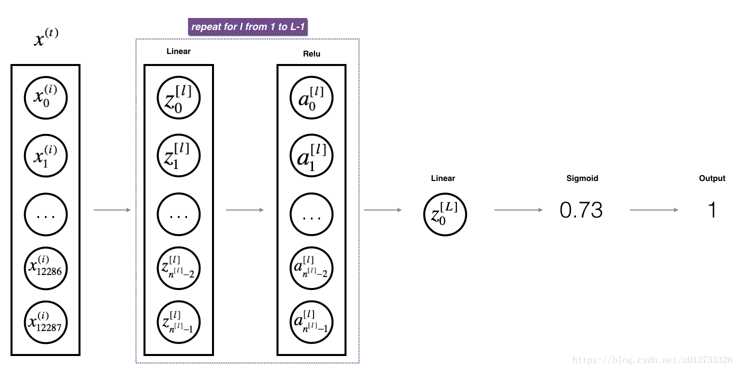
def L_model_forward(X, parameters):'''实现[LINEAR-> RELU] *(L-1) - > LINEAR-> SIGMOID计算前向传播,也就是多层网络的前向传播,为后面每一层都执行LINEAR和ACTIVATION参数:X - 数据,numpy数组,维度为(输入节点数量,示例数)parameters - initialize_parameters_deep()的输出返回:AL - 最后的激活值caches - 包含以下内容的缓存列表:linear_relu_forward()的每个cache(有L-1个,索引为从0到L-2)linear_sigmoid_forward()的cache(只有一个,索引为L-1)'''# 结果存储caches = []A = XL = len(parameters) // 2# 神经网络结构# 前面使用relu激活函数,最后一层使用sigmoid函数for l in range(1, L):A_prev = AA, cache = linear_activation_forward(A_prev, parameters['W'+str(l)], parameters['b'+str(l)], 'relu')caches.append(cache)AL, cache = linear_activation_forward(A, parameters['W'+str(L)],\parameters['b'+str(L)], 'sigmoid')caches.append(cache)# 确保数据格式正确assert(AL.shape == (1, X.shape[1]))return AL, caches测试一下:
#测试L_model_forward
print("==============测试L_model_forward==============")
X,parameters = testCases.L_model_forward_test_case()
AL,caches = L_model_forward(X,parameters)
print("AL = " + str(AL))
print("caches 的长度为 = " + str(len(caches)))
==============测试L_model_forward==============
AL = [[0.17007265 0.2524272 ]]
caches 的长度为 = 2
计算成本
我们已经把这两个模型的前向传播部分完成了,我们需要计算成本(误差),以确定它到底有没有在学习,成本的计算公式如下:
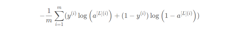
def compute_cost(AL, Y):'''实施等式(4)定义的成本函数。参数:AL - 与标签预测相对应的概率向量,维度为(1,示例数量)Y - 标签向量(例如:如果不是猫,则为0,如果是猫则为1),维度为(1,数量)返回:cost - 交叉熵成本'''# 样本数量mm = Y.shape[1]cost = -np.sum(np.multiply(np.log(AL), Y)+np.multiply(np.log(1-AL),\1-Y))/m# 压缩数据cost = np.squeeze(cost)# 确认数据格式assert(cost.shape == ())return cost
测试一下:
#测试compute_cost
print("==============测试compute_cost==============")
Y,AL = testCases.compute_cost_test_case()
print("cost = " + str(compute_cost(AL, Y)))
==============测试compute_cost==============
cost = 0.414931599615397
反向传播
反向传播用于计算相对于参数的损失函数的梯度,我们来看看向前和向后传播的流程图:
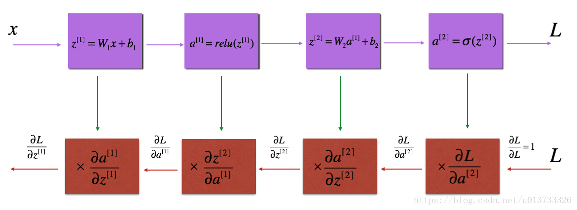
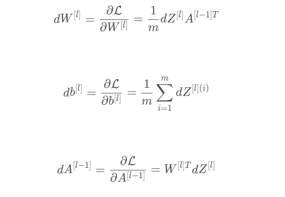
流程图有了,我们再来看一看对于线性的部分的公式:
我们需要使用dZ[l] 来计算三个输出 ( dW[l] , db[l] , dA[l] ) ,下面三个公式是我们要用到的:
与前向传播类似,我们有需要使用三个步骤来构建反向传播:
- LINEAR 后向计算
- LINEAR -> ACTIVATION 后向计算,其中ACTIVATION 计算Relu或者Sigmoid 的结果
- [LINEAR -> RELU] × \times× (L-1) -> LINEAR -> SIGMOID 后向计算 (整个模型)
线性部分【LINEAR backward】
我们来实现后向传播线性部分:
def linear_backward(dZ, cache):'''为单层实现反向传播的线性部分(第L层)参数:dZ - 相对于(当前第l层的)线性输出的成本梯度cache - 来自当前层前向传播的值的元组(A_prev,W,b)返回:dA_prev - 相对于激活(前一层l-1)的成本梯度,与A_prev维度相同dW - 相对于W(当前层l)的成本梯度,与W的维度相同db - 相对于b(当前层l)的成本梯度,与b维度相同'''A_prev, W, b = cachem = A_prev.shape[1]dW = np.dot(dZ, A_prev.T) / mdb = np.sum(dZ, axis=1, keepdims=True) / mdA_prev = np.dot(W.T, dZ)# 确认数据格式正确assert(dA_prev.shape == A_prev.shape)assert(dW.shape == W.shape)assert(db.shape == b.shape)return dA_prev, dW, db
测试一下:
#测试linear_backward
print("==============测试linear_backward==============")
dZ, linear_cache = testCases.linear_backward_test_case()dA_prev, dW, db = linear_backward(dZ, linear_cache)
print ("dA_prev = "+ str(dA_prev))
print ("dW = " + str(dW))
print ("db = " + str(db))
==============测试linear_backward==============
dA_prev = [[ 0.51822968 -0.19517421][-0.40506361  0.15255393][ 2.37496825 -0.89445391]]
dW = [[-0.10076895  1.40685096  1.64992505]]
db = [[0.50629448]]
线性激活部分【LINEAR -> ACTIVATION backward】
为了帮助你实现linear_activation_backward,我们提供了两个后向函数:
- sigmoid_backward:实现了sigmoid()函数的反向传播
- relu_backward: 实现了relu()函数的反向传播
def linear_activation_backward(dA, cache, activation='relu'):'''实现LINEAR-> ACTIVATION层的后向传播。参数:dA - 当前层l的激活后的梯度值cache - 我们存储的用于有效计算反向传播的值的元组(值为linear_cache,activation_cache)activation - 要在此层中使用的激活函数名,字符串类型,【"sigmoid" | "relu"】返回:dA_prev - 相对于激活(前一层l-1)的成本梯度值,与A_prev维度相同dW - 相对于W(当前层l)的成本梯度值,与W的维度相同db - 相对于b(当前层l)的成本梯度值,与b的维度相同'''# 获取参数linear_cache, actvation_cache = cache# 不同的激活函数的导数也不同if activation == 'relu':dZ = relu_backward(dA, actvation_cache)dA_prev, dW, db = linear_backward(dZ, linear_cache)elif activation == 'sigmoid':dZ = sigmoid_backward(dA, actvation_cache)dA_prev, dW, db = linear_backward(dZ, linear_cache)return dA_prev, dW, db
测试一下:
#测试linear_activation_backward
print("==============测试linear_activation_backward==============")
AL, linear_activation_cache = testCases.linear_activation_backward_test_case()dA_prev, dW, db = linear_activation_backward(AL, linear_activation_cache, activation = "sigmoid")
print ("sigmoid:")
print ("dA_prev = "+ str(dA_prev))
print ("dW = " + str(dW))
print ("db = " + str(db) + "\n")dA_prev, dW, db = linear_activation_backward(AL, linear_activation_cache, activation = "relu")
print ("relu:")
print ("dA_prev = "+ str(dA_prev))
print ("dW = " + str(dW))
print ("db = " + str(db))
==============测试linear_activation_backward==============
sigmoid:
dA_prev = [[ 0.11017994  0.01105339][ 0.09466817  0.00949723][-0.05743092 -0.00576154]]
dW = [[ 0.10266786  0.09778551 -0.01968084]]
db = [[-0.05729622]]relu:
dA_prev = [[ 0.44090989 -0.        ][ 0.37883606 -0.        ][-0.2298228   0.        ]]
dW = [[ 0.44513824  0.37371418 -0.10478989]]
db = [[-0.20837892]]
构建多层模型向后传播函数
def L_model_backward(AL, Y, caches):'''对[LINEAR-> RELU] *(L-1) - > LINEAR - > SIGMOID组执行反向传播,就是多层网络的向后传播参数:AL - 概率向量,正向传播的输出(L_model_forward())Y - 标签向量(例如:如果不是猫,则为0,如果是猫则为1),维度为(1,数量)caches - 包含以下内容的cache列表:linear_activation_forward("relu")的cache,不包含输出层linear_activation_forward("sigmoid")的cache返回:grads - 具有梯度值的字典grads [“dA”+ str(l)] = ...grads [“dW”+ str(l)] = ...grads [“db”+ str(l)] = ...'''# 初始化参数grads = {
    }L = len(caches)m = AL.shape[1]Y = Y.reshape(AL.shape)dAL = -(np.divide(Y, AL)-np.divide(1-Y, 1-AL))current_cache = caches[L-1]grads['dA'+str(L)], grads['dW'+str(L)], grads['db'+str(L)] = \linear_activation_backward(dAL, current_cache, 'sigmoid')# 逐层进行反向传播for l in reversed(range(L-1)):current_cache = caches[l]  #当前层dA_prev_temp, dW_temp, db_temp = linear_activation_backward(grads['dA'+\str(l+2)], current_cache, 'relu')grads['dA'+str(l+1)] = dA_prev_tempgrads['dW'+str(l+1)] = dW_tempgrads['db'+str(l+1)] = db_tempreturn grads
测试一下:
#测试L_model_backward
print("==============测试L_model_backward==============")
AL, Y_assess, caches = testCases.L_model_backward_test_case()
grads = L_model_backward(AL, Y_assess, caches)
print ("dW1 = "+ str(grads["dW1"]))
print ("db1 = "+ str(grads["db1"]))
print ("dA1 = "+ str(grads["dA1"]))
==============测试L_model_backward==============
dW1 = [[0.41010002 0.07807203 0.13798444 0.10502167][0.         0.         0.         0.        ][0.05283652 0.01005865 0.01777766 0.0135308 ]]
db1 = [[-0.22007063][ 0.        ][-0.02835349]]
dA1 = [[ 0.          0.52257901][ 0.         -0.3269206 ][ 0.         -0.32070404][ 0.         -0.74079187]]
更新参数
我们把向前向后传播都完成了,现在我们就开始更新参数,当然,我们来看看更新参数的公式吧~
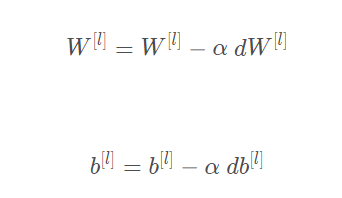
其中α是学习率。
def update_parameters(parameters, grads, learning_rate):'''使用梯度下降更新参数参数:parameters - 包含你的参数的字典grads - 包含梯度值的字典,是L_model_backward的输出返回:parameters - 包含更新参数的字典参数[“W”+ str(l)] = ...参数[“b”+ str(l)] = ...'''# 获取隐藏层数L = len(parameters) // 2# 逐层进行更新for l in range(L):parameters['W'+str(l+1)] = parameters['W'+str(l+1)]-learning_rate*\grads["dW" + str(l + 1)]parameters['b'+str(l+1)] = parameters['b'+str(l+1)]-learning_rate*\grads['db'+str(l+1)]return parameters
测试一下:
#测试update_parameters
print("==============测试update_parameters==============")
parameters, grads = testCases.update_parameters_test_case()
parameters = update_parameters(parameters, grads, 0.1)print ("W1 = "+ str(parameters["W1"]))
print ("b1 = "+ str(parameters["b1"]))
print ("W2 = "+ str(parameters["W2"]))
print ("b2 = "+ str(parameters["b2"]))
==============测试update_parameters==============
W1 = [[-0.59562069 -0.09991781 -2.14584584  1.82662008][-1.76569676 -0.80627147  0.51115557 -1.18258802][-1.0535704  -0.86128581  0.68284052  2.20374577]]
b1 = [[-0.04659241][-1.28888275][ 0.53405496]]
W2 = [[-0.55569196  0.0354055   1.32964895]]
b2 = [[-0.84610769]]
搭建两层神经网络
一个两层的神经网络模型图如下:
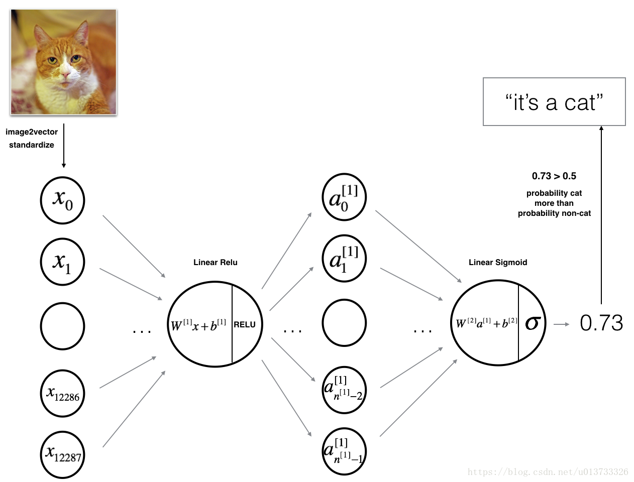
该模型可以概括为: INPUT -> LINEAR -> RELU -> LINEAR -> SIGMOID -> OUTPUT
我们正式开始构建两层的神经网络:
def two_layer_model(X, Y, layers_dims, learning_rate=0.0075, \num_iterations=3000, print_cost=False, isPlot=True):'''实现一个两层的神经网络,【LINEAR->RELU】 -> 【LINEAR->SIGMOID】参数:X - 输入的数据,维度为(n_x,例子数)Y - 标签,向量,0为非猫,1为猫,维度为(1,数量)layers_dims - 层数的向量,维度为(n_y,n_h,n_y)learning_rate - 学习率num_iterations - 迭代的次数print_cost - 是否打印成本值,每100次打印一次isPlot - 是否绘制出误差值的图谱返回:parameters - 一个包含W1,b1,W2,b2的字典变量'''# 设置随机种子,保证结果可复现np.random.seed(1)'''初始化参数'''grads = {
    }costs = [](n_x, n_h, n_y) = layers_dimsparameters = initialize_parameters(n_x, n_h, n_y)W1 = parameters['W1']b1 = parameters['b1']W2 = parameters['W2']b2 = parameters['b2']# 开始进行迭代for i in range(num_iterations):# 前向传播A1, cache1 = linear_activation_forward(X, W1, b1, 'relu')A2, cache2 = linear_activation_forward(A1, W2, b2, 'sigmoid')# 计算成本cost = compute_cost(A2, Y)# 后向传播# 初始化后向传播dA2 = -(np.divide(Y, A2) - np.divide(1-Y, 1-A2))# 后向传播dA1, dW2, db2 = linear_activation_backward(dA2, cache2, 'sigmoid')dA0, dW1, db1 = linear_activation_backward(dA1, cache1, 'relu')# 向后传播的数据保存到gradsgrads['dW1'] = dW1grads['db1'] = db1grads['dW2'] = dW2grads['db2'] = db2# 更新参数parameters = update_parameters(parameters, grads, learning_rate)W1 = parameters['W1']b1 = parameters['b1']W2 = parameters['W2']b2 = parameters['b2']# 打印成本值,如果print_cost=False则被忽略if i%100 == 0:#记录成本costs.append(cost)if print_cost:print('第',i,'次迭代,成本值为:', np.squeeze(cost))#迭代完成,则根据条件进行绘制图if isPlot:plt.plot(np.squeeze(costs))plt.ylabel('cost')plt.xlabel('iterations (per tens)')plt.title('Learing rate = '+str(learning_rate))plt.show()# 返回参数parametersreturn parameters
加载数据集,开始训练
train_set_x_orig , train_set_y , test_set_x_orig , test_set_y , classes = lr_utils.load_dataset()train_x_flatten = train_set_x_orig.reshape(train_set_x_orig.shape[0], -1).T
test_x_flatten = test_set_x_orig.reshape(test_set_x_orig.shape[0], -1).Ttrain_x = train_x_flatten / 255
train_y = train_set_y
test_x = test_x_flatten / 255
test_y = test_set_yn_x = 12288
n_h = 7
n_y = 1
layers_dims = (n_x,n_h,n_y)parameters = two_layer_model(train_x, train_set_y, layers_dims = (n_x, n_h, n_y), num_iterations = 2500, print_cost=True,isPlot=True)
第 0 次迭代,成本值为: 0.6930497356599891
第 100 次迭代,成本值为: 0.6464320953428849
第 200 次迭代,成本值为: 0.6325140647912677
第 300 次迭代,成本值为: 0.6015024920354665
第 400 次迭代,成本值为: 0.5601966311605748
第 500 次迭代,成本值为: 0.515830477276473
第 600 次迭代,成本值为: 0.47549013139433266
第 700 次迭代,成本值为: 0.43391631512257495
第 800 次迭代,成本值为: 0.400797753620389
第 900 次迭代,成本值为: 0.3580705011323798
第 1000 次迭代,成本值为: 0.3394281538366412
第 1100 次迭代,成本值为: 0.3052753636196264
第 1200 次迭代,成本值为: 0.2749137728213017
第 1300 次迭代,成本值为: 0.2468176821061485
第 1400 次迭代,成本值为: 0.19850735037466108
第 1500 次迭代,成本值为: 0.174483181125566
第 1600 次迭代,成本值为: 0.17080762978096897
第 1700 次迭代,成本值为: 0.11306524562164709
第 1800 次迭代,成本值为: 0.09629426845937147
第 1900 次迭代,成本值为: 0.08342617959726864
第 2000 次迭代,成本值为: 0.07439078704319083
第 2100 次迭代,成本值为: 0.06630748132267932
第 2200 次迭代,成本值为: 0.05919329501038171
第 2300 次迭代,成本值为: 0.05336140348560558
第 2400 次迭代,成本值为: 0.0485547856287702
[外链图片转存失败,源站可能有防盗链机制,建议将图片保存下来直接上传(img-wPFkinsw-1630572037364)(output_48_1.png)]
构建预测函数
def predict(X, y, parameters):'''该函数用于预测L层神经网络的结果,当然也包含两层参数:X - 测试集y - 标签parameters - 训练模型的参数返回:p - 给定数据集X的预测'''# 获取样本数量mm = X.shape[1]n = len(parameters) // 2 #神经网络的层数p = np.zeros((1, m))# 根据参数向前传播probas, caches = L_model_forward(X, parameters)# 进行预测for i in range(0, probas.shape[1]):# 界限是0.5if probas[0, i] > 0.5:p[0, i] = 1else:p[0, i] = 0print("准确度为:"+str(float(np.sum((p==y))/m)))return p
查看训练集和测试集的准确性
predictions_train = predict(train_x, train_y, parameters)
predictions_test = predict(test_x, test_y, parameters)
准确度为:1.0
准确度为:0.72
搭建多层神经网络
我们首先来看看多层的网络的结构吧~
def L_layer_model(X, Y, layers_dims, learning_rate=0.0075, num_iterations=3000,\print_cost=False, isPlot=False):'''实现一个L层神经网络:[LINEAR-> RELU] *(L-1) - > LINEAR-> SIGMOID。参数:X - 输入的数据,维度为(n_x,例子数)Y - 标签,向量,0为非猫,1为猫,维度为(1,数量)layers_dims - 层数的向量,维度为(n_y,n_h,・・・,n_h,n_y)learning_rate - 学习率num_iterations - 迭代的次数print_cost - 是否打印成本值,每100次打印一次isPlot - 是否绘制出误差值的图谱返回:parameters - 模型学习的参数。 然后他们可以用来预测。'''# 设置随机数种子,保证结果一致性np.random.seed(1)costs = []# 随机初始化网络参数parameters = initialize_parameters_deep(layers_dims)for i in range(0, num_iterations):# 前向传播AL, caches = L_model_forward(X, parameters)# 计算代价函数cost = compute_cost(AL, Y)# 反向传播grads = L_model_backward(AL, Y, caches)# 梯度下降parameters = update_parameters(parameters, grads, learning_rate)#打印成本值,如果print_cost = False则省略if i%100 == 0:# 记录成本costs.append(cost)# 是否打印成本值if print_cost:print("第",i,"次迭代,成本值为:", np.squeeze(cost))# 迭代完成,根据条件绘制图if isPlot:plt.plot(np.squeeze(costs))plt.ylabel('cost')plt.xlabel('iterations (per tens)')plt.title('Learning rate = '+str(learning_rate))plt.show()return parameters
继续进行模型训练和测试
train_set_x_orig , train_set_y , test_set_x_orig , test_set_y , classes = lr_utils.load_dataset()train_x_flatten = train_set_x_orig.reshape(train_set_x_orig.shape[0], -1).T
test_x_flatten = test_set_x_orig.reshape(test_set_x_orig.shape[0], -1).Ttrain_x = train_x_flatten / 255
train_y = train_set_y
test_x = test_x_flatten / 255
test_y = test_set_y# 正式训练
layers_dims = [12288, 20, 7, 5, 1] # 5-layer model
parameters = L_layer_model(train_x, train_y, layers_dims, num_iterations = 2500, print_cost = True,isPlot=True)
第 0 次迭代,成本值为: 0.715731513413713
第 100 次迭代,成本值为: 0.6747377593469114
第 200 次迭代,成本值为: 0.6603365433622128
第 300 次迭代,成本值为: 0.6462887802148751
第 400 次迭代,成本值为: 0.6298131216927773
第 500 次迭代,成本值为: 0.6060056229265339
第 600 次迭代,成本值为: 0.5690041263975134
第 700 次迭代,成本值为: 0.519796535043806
第 800 次迭代,成本值为: 0.46415716786282285
第 900 次迭代,成本值为: 0.40842030048298916
第 1000 次迭代,成本值为: 0.37315499216069037
第 1100 次迭代,成本值为: 0.3057237457304712
第 1200 次迭代,成本值为: 0.2681015284774084
第 1300 次迭代,成本值为: 0.23872474827672593
第 1400 次迭代,成本值为: 0.20632263257914712
第 1500 次迭代,成本值为: 0.17943886927493546
第 1600 次迭代,成本值为: 0.15798735818801213
第 1700 次迭代,成本值为: 0.1424041301227393
第 1800 次迭代,成本值为: 0.12865165997885838
第 1900 次迭代,成本值为: 0.11244314998155497
第 2000 次迭代,成本值为: 0.08505631034966696
第 2100 次迭代,成本值为: 0.05758391198605791
第 2200 次迭代,成本值为: 0.0445675345469387
第 2300 次迭代,成本值为: 0.03808275166597669
第 2400 次迭代,成本值为: 0.034410749018403054
[外链图片转存失败,源站可能有防盗链机制,建议将图片保存下来直接上传(img-aW3187qo-1630572037365)(output_56_1.png)]
# 预测
pred_train = predict(train_x, train_y, parameters) #训练集
pred_test = predict(test_x, test_y, parameters) #测试集
准确度为:0.9952153110047847
准确度为:0.78
就准确度而言,从70%到72%再到78%,可以看到的是准确度在一点点增加,当然,你也可以手动的去调整layers_dims,准确度可能又会提高一些。
分析
我们可以看看有哪些东西在L层模型中被错误地标记了,导致准确率没有提高
def print_mislabeled_images(classes, X, y, p):'''绘制预测和实际不同的图像。X - 数据集y - 实际的标签p - 预测'''a = p+y# 错误分类的是a==1,有两种情况p=0,y=1或p=1,y=0mislabeled_indices = np.asarray(np.where(a == 1))plt.rcParams['figure.figsize'] = (40.0, 40.0) #设置默认的图片大小num_images = len(mislabeled_indices[0])for i in range(num_images):# 找到错误的图像index = mislabeled_indices[1][i]plt.subplot(2, num_images, i+1)# Matplotlib库中,调用imshow()函数实现热图绘制。# 参数:interpolation 用于设置使用的插值方法plt.imshow(X[:,index].reshape(64, 64,3), interpolation='nearest')plt.axis('off')plt.title('Prediction:'+classes[int(p[0, index])].decode('utf-8'))print_mislabeled_images(classes, test_x, test_y, pred_test)
[外链图片转存失败,源站可能有防盗链机制,建议将图片保存下来直接上传(img-B14b1Tih-1630572037366)(output_59_0.png)]
分析一下我们就可以得知原因了:
模型往往表现欠佳的几种类型的图像包括:
- 猫身体在一个不同的位置
- 猫出现在相似颜色的背景下
- 不同的猫的颜色和品种
- 相机角度
- 图片的亮度
- 比例变化(猫的图像非常大或很小)
【选做】
我们使用自己图片试试?
我们把一张图片放在一个特定位置,然后识别它。
from PIL import Image
my_image = "my_image.png" # change this to the name of your image file
my_label_y = [1]fname =  "images/" + my_image
num_px = 64
# 读取图片,将其转化为三通道,并resize为64*64分辨率
image = Image.open(fname).convert("RGB").resize((num_px, num_px))
# 将图片转化为矩阵形式并reshape以满足模型输入格式my_image = np.array(image).reshape(num_px * num_px * 3, -1)my_predict_image = predict(my_image,my_label_y,parameters)
plt.imshow(image)
准确度为:1.0<matplotlib.image.AxesImage at 0x2afb5884788>
[外链图片转存失败,源站可能有防盗链机制,建议将图片保存下来直接上传(img-Lk0A8m2c-1630572037366)(output_62_2.png)]
相关库代码
lr_utils.py
# lr_utils.py
import numpy as np
import h5pydef load_dataset():train_dataset = h5py.File('datasets/train_catvnoncat.h5', "r")train_set_x_orig = np.array(train_dataset["train_set_x"][:]) # your train set featurestrain_set_y_orig = np.array(train_dataset["train_set_y"][:]) # your train set labelstest_dataset = h5py.File('datasets/test_catvnoncat.h5', "r")test_set_x_orig = np.array(test_dataset["test_set_x"][:]) # your test set featurestest_set_y_orig = np.array(test_dataset["test_set_y"][:]) # your test set labelsclasses = np.array(test_dataset["list_classes"][:]) # the list of classestrain_set_y_orig = train_set_y_orig.reshape((1, train_set_y_orig.shape[0]))test_set_y_orig = test_set_y_orig.reshape((1, test_set_y_orig.shape[0]))return train_set_x_orig, train_set_y_orig, test_set_x_orig, test_set_y_orig, classes
dnn_utils.py
# dnn_utils.py
import numpy as npdef sigmoid(Z):"""Implements the sigmoid activation in numpyArguments:Z -- numpy array of any shapeReturns:A -- output of sigmoid(z), same shape as Zcache -- returns Z as well, useful during backpropagation"""A = 1/(1+np.exp(-Z))cache = Zreturn A, cachedef sigmoid_backward(dA, cache):"""Implement the backward propagation for a single SIGMOID unit.Arguments:dA -- post-activation gradient, of any shapecache -- 'Z' where we store for computing backward propagation efficientlyReturns:dZ -- Gradient of the cost with respect to Z"""Z = caches = 1/(1+np.exp(-Z))dZ = dA * s * (1-s)assert (dZ.shape == Z.shape)return dZdef relu(Z):"""Implement the RELU function.Arguments:Z -- Output of the linear layer, of any shapeReturns:A -- Post-activation parameter, of the same shape as Zcache -- a python dictionary containing "A" ; stored for computing the backward pass efficiently"""A = np.maximum(0,Z)assert(A.shape == Z.shape)cache = Z return A, cachedef relu_backward(dA, cache):"""Implement the backward propagation for a single RELU unit.Arguments:dA -- post-activation gradient, of any shapecache -- 'Z' where we store for computing backward propagation efficientlyReturns:dZ -- Gradient of the cost with respect to Z"""Z = cachedZ = np.array(dA, copy=True) # just converting dz to a correct object.# When z <= 0, you should set dz to 0 as well. dZ[Z <= 0] = 0assert (dZ.shape == Z.shape)return dZ
testCase.py
#testCase.py
import numpy as npdef linear_forward_test_case():np.random.seed(1)A = np.random.randn(3,2)W = np.random.randn(1,3)b = np.random.randn(1,1)return A, W, bdef linear_activation_forward_test_case():np.random.seed(2)A_prev = np.random.randn(3,2)W = np.random.randn(1,3)b = np.random.randn(1,1)return A_prev, W, bdef L_model_forward_test_case():np.random.seed(1)X = np.random.randn(4,2)W1 = np.random.randn(3,4)b1 = np.random.randn(3,1)W2 = np.random.randn(1,3)b2 = np.random.randn(1,1)parameters = {
    "W1": W1,"b1": b1,"W2": W2,"b2": b2}return X, parametersdef compute_cost_test_case():Y = np.asarray([[1, 1, 1]])aL = np.array([[.8,.9,0.4]])return Y, aLdef linear_backward_test_case():np.random.seed(1)dZ = np.random.randn(1,2)A = np.random.randn(3,2)W = np.random.randn(1,3)b = np.random.randn(1,1)linear_cache = (A, W, b)return dZ, linear_cachedef linear_activation_backward_test_case():np.random.seed(2)dA = np.random.randn(1,2)A = np.random.randn(3,2)W = np.random.randn(1,3)b = np.random.randn(1,1)Z = np.random.randn(1,2)linear_cache = (A, W, b)activation_cache = Zlinear_activation_cache = (linear_cache, activation_cache)return dA, linear_activation_cachedef L_model_backward_test_case():np.random.seed(3)AL = np.random.randn(1, 2)Y = np.array([[1, 0]])A1 = np.random.randn(4,2)W1 = np.random.randn(3,4)b1 = np.random.randn(3,1)Z1 = np.random.randn(3,2)linear_cache_activation_1 = ((A1, W1, b1), Z1)A2 = np.random.randn(3,2)W2 = np.random.randn(1,3)b2 = np.random.randn(1,1)Z2 = np.random.randn(1,2)linear_cache_activation_2 = ( (A2, W2, b2), Z2)caches = (linear_cache_activation_1, linear_cache_activation_2)return AL, Y, cachesdef update_parameters_test_case():np.random.seed(2)W1 = np.random.randn(3,4)b1 = np.random.randn(3,1)W2 = np.random.randn(1,3)b2 = np.random.randn(1,1)parameters = {
    "W1": W1,"b1": b1,"W2": W2,"b2": b2}np.random.seed(3)dW1 = np.random.randn(3,4)db1 = np.random.randn(3,1)dW2 = np.random.randn(1,3)db2 = np.random.randn(1,1)grads = {
    "dW1": dW1,"db1": db1,"dW2": dW2,"db2": db2}return parameters, grads