DGM: A deep learning algorithm for solving partial differential equations_综合

论文信息

题目：DGM: A deep learning algorithm for solving partial differential equations

作者：Justin Sirignano? and Konstantinos Spiliopoulos

期刊、会议：

单位：

时间：18

代码：

基础

论文动机

High-dimensional partial differential equations (PDEs) are used in physics, engineering, and finance. Their numerical solution has been a longstanding challenge
This quickly becomes computationally intractable when the dimension d becomes even moderately large. We propose to solve high-dimensional PDEs using a meshfree deep learning algorithm.
The method is similar in spirit to the Galerkin method, but with several key changes using ideas from machine learning.
The Galerkin method is a widely-used computational method which seeks a reduced-form solution to a PDE as a linear combinationof basis functions.
DGM is a natural merger of Galerkin methods and machine learning

本文方法

Approximation Power of Neural Networks for PDEs

$?tu(t,x)+Lu(t,x)=0,(t,x)∈[0,T]×Ωu(0,x)=u0(x),x∈Ωu(t,x)=g(t,x),x∈[0,T]×?Ω\begin{array}{ll} \partial_{t} u(t, x)+\mathcal{L} u(t, x)=0, & (t, x) \in[0, T] \times \Omega \\ u(0, x)=u_{0}(x), & x \in \Omega \\ u(t, x)=g(t, x), & x \in[0, T] \times \partial \Omega \end{array}$

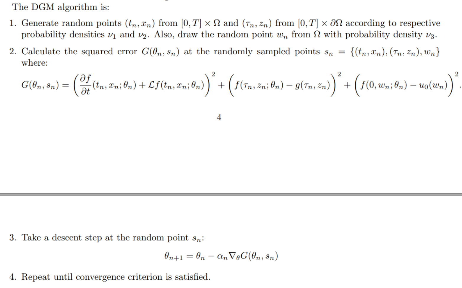
The error function:
$J(f)=∥?tf+Lf∥2,[0,T]×Ω2+∥f?g∥2,[0,T]×?Ω2+∥f(0,?)?u0∥2,Ω2J(f)=\left\|\partial_{t} f+\mathcal{L} f\right\|_{2,[0, T] \times \Omega}^{2}+\|f-g\|_{2,[0, T] \times \partial \Omega}^{2}+\left\|f(0, \cdot)-u_{0}\right\|_{2, \Omega}^{2}$

This paper explores several new innovations：

First, we focus on high-dimensional PDEs and apply deep learning advances of the past decade to this problem.
Secondly, to avoid ever forming a mesh, we sample a sequence of random spatial points.
Thirdly, the algorithm incorporates a new computational scheme for the efficient computationof neural network gradients arising from the second derivatives of high-dimensional PDEs.

DGM

在这里插入图片描述

A Monte Carlo Method for Fast Computation of Second Derivatives

The computational cost for calculating second derivatives

在这里插入图片描述
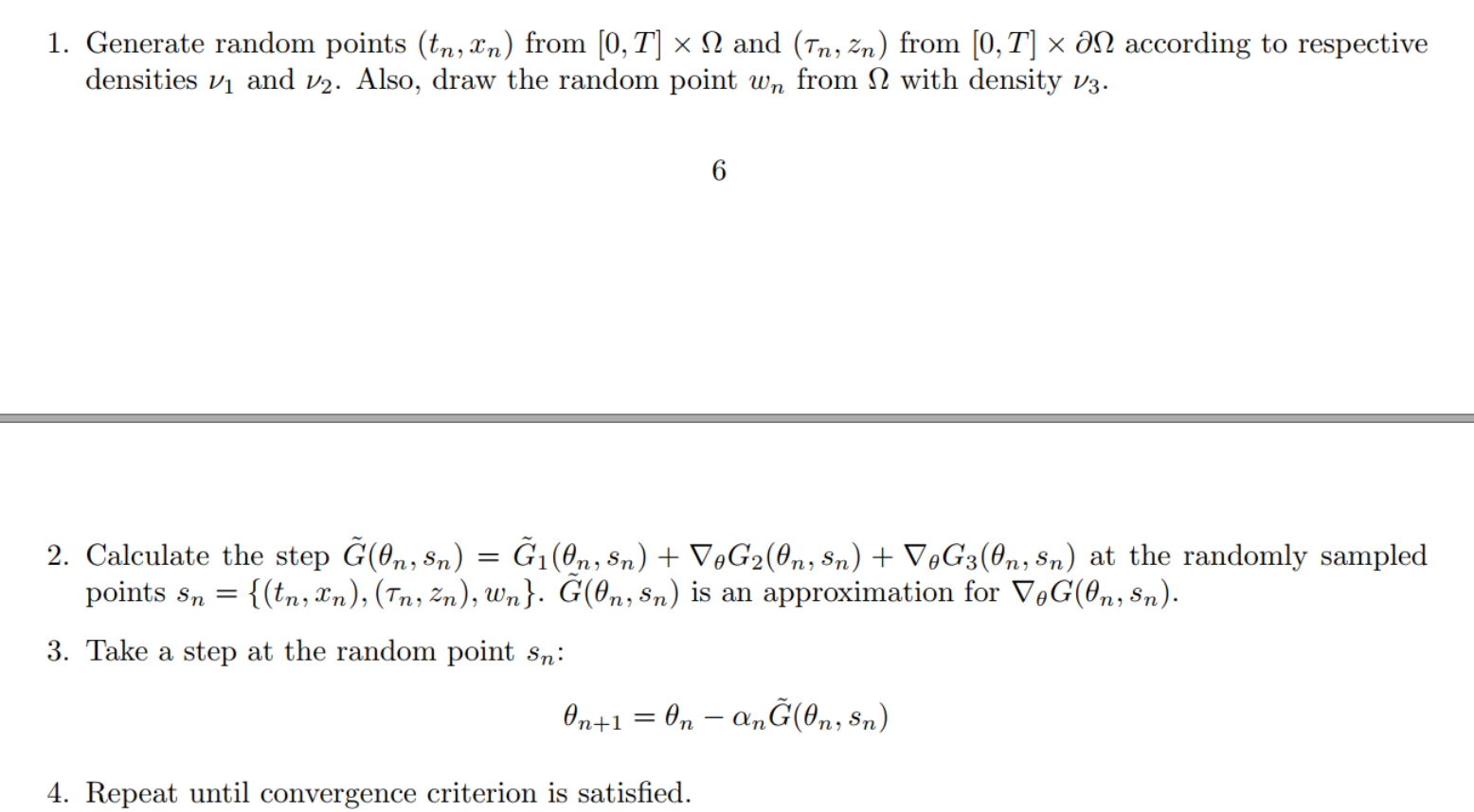
The modified algorithm here is computationally less expensive than the original algorithm

Relevant literature

Recently, Raissi [41, 42] develop physics informed deep learning models. They estimate deep neural network models which merge data observations with PDE models. This allows for the estimation of physical models from limited data by leveraging a priori knowledge that the physical dynamics should obey a class of PDEs. Their approach solves PDEs in one and two spatial dimensions using deep neural networks.
[33] developed an algorithm for the solution of a discrete-time version of a class of free boundary PDEs.
Their algorithm, commonly called the Longstaff-Schwartz method", uses dynamic programming and approximates the solution using a separate function approximator at each discrete time (typically a linear combination of basis functions). Our algorithm directly solves the PDE, and uses a single function approximator for all space and all time.

DGM: A deep learning algorithm for solving partial differential equations