[论文翻译]A Global Geometric Framework for Nonlinear Dimensionality Reduction

论文题目：A Global Geometric Framework for Nonlinear Dimensionality Reduction
论文来源:Science 290, 2319 (2000);

A Global Geometric Framework for Nonlinear Dimensionality Reduction

非线性降维的全局几何框架

Joshua B. Tenenbaum,^1* Vin de Silva,² John C. Langford³

Scientists working with large volumes of high-dimensional data, such as global climate patterns, stellar spectra, or human gene distributions, regularly confront the problem of dimensionality reduction: ?nding meaningful low-dimensional structures hidden in their high-dimensional observations. The human brain confronts the same problem in everyday perception, extracting from its high-dimensional sensory inputs—30,000 auditory nerve ?bers or 106 optic nerve ?bers—a manageably small number of perceptually relevant features. Here we describe an approach to solving dimensionality reduction problems that uses easily measured local metric information to learn the underlying global geometry of a data set. Unlike classical techniques such as principal component analysis (PCA) and multidimensional scaling (MDS), our approach is capable of discovering the nonlinear degrees of freedom that underlie complex natural observations,such as human handwriting or images of a face under different viewing conditions. In contrast to previous algorithms for nonlinear dimensionality reduction,our sef?ciently computes a globally optimal solution, and, for an important class of data manifolds, is guaranteed to converge asymptotically to the true structure.

科学家们在处理大量高维数据时，如全球气候模式、恒星光谱或人类基因分布等，经常会面临维度降低的问题：在高维观测过程中，发现隐藏在其中的有意义的低维结构。人脑在日常感知中也面临同样的问题，从高维感官输入中提取出30,000个听觉神经元或106个视神经纤维，这是数量很少的感知相关特征。在这里，我们描述了一种解决维度降低问题的方法，该方法使用易于测量的局部度量信息来学习数据集的底层全局几何，与主成分分析(PCA)和多维度缩放(MDS)等经典技术不同，我们的方法能够发现复杂的自然观察结果所蕴含的非线性自由度，例如不同观察条件下的人类笔迹或人脸图像。与以往的非线性维度降低算法相比，我们的方法能够计算出一个全局最优的解，并且对于一类重要的数据表征，保证渐进地收敛到真实结构。

A canonical problem in dimensionality reduction from the domain of visual perception is illustrated in Fig. 1A. The input consists of many images of a person’s face observed under different pose and lighting conditions, in no particular order. These images can be thought of as points in a high-dimensional vector space, with each input dimension corresponding to the brightness of one pixel in the image or the firing rate of one retinal ganglion cell. Although the input dimensionality may be quite high (e.g., 4096 for these 64 pixel by 64 pixel images), the perceptually meaningful structure of these images has many fewer independent degrees of freedom. Within the 4096-dimensional input space, all of the images lie on an intrinsically three dimensional manifold, or constraint surface, that can be parameterized by two pose variables plus an azimuthal lighting angle. Our goal is to discover, given only the unordered high-dimensional inputs, low-dimensional representations such as Fig. 1A with coordinates that capture the intrinsic degrees of freedom of a data set. This problem is of central importance not only in studies of vision (1–5), but also in speech (6, 7), motor control (8, 9), and a range of other physical and biological sciences (10–12).

图1的A是视觉感知领域的一个典型的维度降低问题。输入包含在不同姿势和光照条件下以特定顺序观察到的许多人脸图像。这些图像可以被认为是高维向量空间中的点，每个输入维度对应图像中一个像素的亮度或一个视网膜神经节细胞的放电率。虽然输入维度可能相当高，例如，对于这些64x64像素的图像来说，为4096，但这些图像的感知意义结构具有较少的独立自由度。在4096维的输入空间内，所有的图像都位于一个本质上的三维面，或者说约束面，它可以由两个姿势变量加上一个方位光照角进行参数化。我们的目标是，只给定无序的高维输入，发现如图1中的A这样的低维表示，其坐标可以捕捉数据集的固有自由度。这个问题不仅在视觉(1-5)的研究中具有核心重要性，而且在语音(6，7)、运动控制(8，9)以及一系列其他物理和生物科学(10-12)中也具有核心重要性。

======================================================================================================


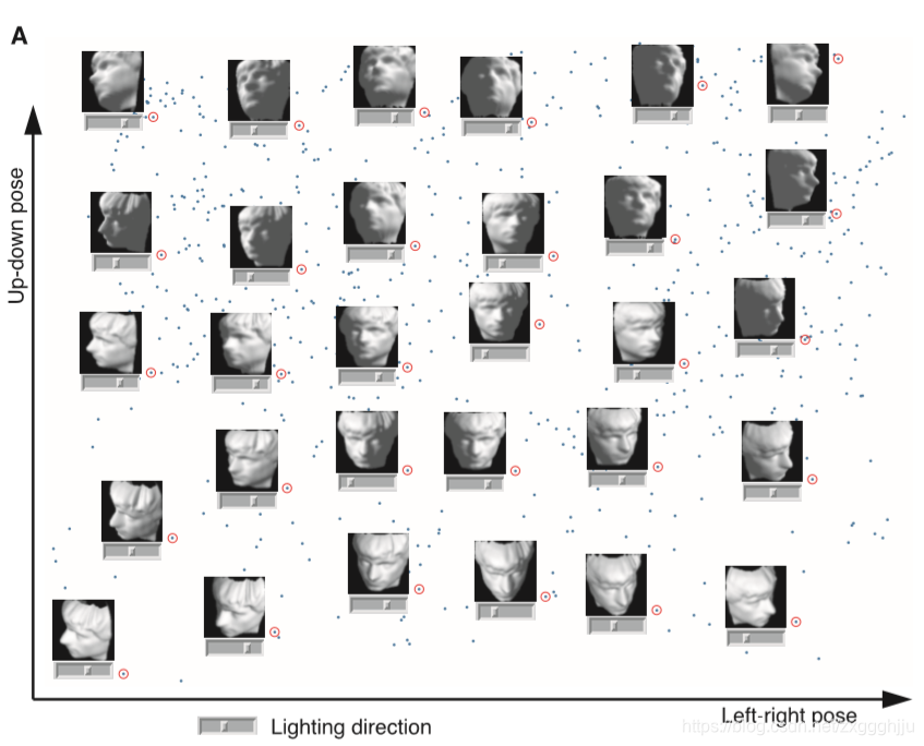
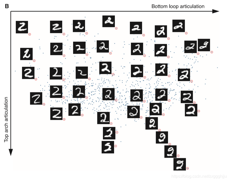
Fig. 1. (A) A canonical dimensionality reduction problem from visual perception.The input consists of a sequence of 4096-dimensional vectors, representing the brightness values of 64 pixel by 64 pixel images of a face rendered with different poses and lighting directions. Applied to N =698 raw images,Isomap(K=6) learns a three-dimension al embedding of the data’s intrinsic geometric structure. A two-dimensional projection is shown, with a sample of the original input images (red circles) superimposed on all the data points (blue) and horizontal sliders (under the images) representing the third dimension. Each coordinate axis of the embedding correlates highly with one degree of freedom underlying the original data: leftright pose (x axis, R =0.99), up-down pose (y axis, R =0.90), and lighting direction (slider position, R =0.92). The input-space distances dx(i,j) given to Isomap were Euclidean distances between the 4096-dimensional image vectors. (B) Isomap applied to N =1000 handwritten “2”s from the MNIST database (40). The two most signi?cant dimensions in the Isomap embedding, shown here, articulate the major features of the “2”: bottom loop (x axis) and top arch (y axis). Input-space distances dx(i,j) were measured by tangent distance,a metric designed to capture the invariances relevant in handwriting recognition (41). Here we used e-Isomap (with ε=4.2) because we did not expect a constant dimensionality to hold over the whole data set; consistent with this, Isomap ?nds several tendrils projecting from the higher dimensional mass of data and representing successive exaggerations of an extra stroke or ornament in the digit.

图1.(A) 一个从视觉感知出发的规范维度降低问题.输入由4096个维度的向量序列组成,代表以不同姿势和光照方向渲染的面部的64像素乘64像素图像的亮度值。应用于N=698张原始图像，Isomap(K=6)可以学习数据内在几何结构的三维嵌入。图中显示了一个二维投影，原始输入图像的样本，即红色圆圈叠加在所有数据点，即蓝色点上，水平滑块（图像下方）代表第三维。嵌入的每个坐标轴与原始数据基础的一个自由度高度相关：左右的姿势（x轴，R=0.99），上下姿势（y轴，R=0.90），以及照明方向（滑块位置，R=0.92）。给予Isomap的输入空间距离dx(i,j)是4096维图像向量之间的欧氏距离。(B) Isomap应用于MNIST数据库(40)中的N =1000个手写 “2”。在Isomap嵌入中的两个最显著的维度，这里显示，阐明了 "2 "的主要特征：底部环（x轴）和顶部拱形（y轴）。输入空间的距离dx(i,j)由切线距离测量，一个旨在捕捉手写识别中相关的不变量的度量(41)。在这里，我们使用e-Isomap（ε=4.2），因为我们并不期望在整个数据集上保持一个恒定的维度；与此一致，Isomap定义了几个从较高维度的数据质量中投射出来的卷须，并代表数字中一个额外笔画或纹饰的连续夸张。

=======================================================================================================
The classical techniques for dimensionality reduction, PCA and MDS, are simple to implement, efficiently computable, and guaranteed to discover the true structure of data lying on or near a linear subspace of the high-dimensional input space (13). PCA finds a low-dimensional embedding of the data points that best preserves their variance as measured in the high-dimensional input space. Classical MDS finds an embedding that preserves the interpoint distances, equivalent to PCA when those distances are Euclidean. However, many data sets contain essential nonlinear structures that are invisible to PCA and MDS (4, 5, 11, 14). For example, both methods fail to detect the true degrees of freedom of the face data set (Fig. 1A), or even its intrinsic three-dimensionality (Fig. 2A).

经典的降维技术PCA和MDS，实现简单，计算效率高，并保证发现躺在高维输入空间的线性子空间上或附近的数据的真实结构（13）。PCA发现了一个低维数据点的嵌入，它能最好地保留数据点在高维输入空间中的方差。经典MDS找到一个能保存点间距离的嵌入，当这些距离是欧几里得时，相当于PCA。然而，许多数据集包含重要的非线性结构，而这些结构是PCA和MDS所看不到的（4，5，11，14）。例如，这两种方法都无法检测到人脸数据集的真实自由度（图1A），甚至无法检测到其固有的三维性（图2A）。

Here we describe an approach that combines the major algorithmic features of PCA and MDS—computational efficiency, global optimality, and asymptotic convergence guarantees—with the flexibility to learn a broad class of nonlinear manifolds. Figure 3 A illustrates the challenge of nonlinearity with data lying on a two-dimensional “Swiss roll”: points far apart on the underlying manifold, as measured by their geodesic, or shortest path, distances, may appear deceptively close in the high-dimensional input space, as measured by their straight-line Euclidean distance. Only the geodesic distances reflect the true low-dimensional geometry of the manifold, but PCA and MDS effectively see just the Euclidean structure; thus, they fail to detect the intrinsic twodimensionality (Fig. 2B).

在这里，我们描述了一种方法，它结合了PCA和MDS的主要算法特征：计算效率、全局优化和渐进收敛保证，以及学习广泛的非线性流形的灵活性。图3的A说明了在二维 "瑞士卷 "上的非线性数据所面临的挑战：在底层流形上相距甚远的点，按照它们的测地线或最短路径的距离来衡量，在高维输入空间中，按照它们的欧氏直线距离来衡量，可能会显得非常接近。只有测地距离才反映了真正的低维几何学，但PCA和MDS实际上只看到了欧氏结构；因此，它们无法检测内在的二维性（图2B）。

Our approach builds on classical MDS but seeks to preserve the intrinsic geometry of the data, as captured in the geodesic manifold distances between all pairs of data points. The crux is estimating the geodesic distance between faraway points, given only input-space distances. For neighboring points, inputspace distance provides a good approximation to geodesic distance. For faraway points, geodesic distance can be approximated by adding up a sequence of “short hops” between neighboring points. These approximations are computed efficiently by finding shortest paths in a graph with edges connecting neighboring data points.

我们的方法建立在经典MDS的基础上，但力求保留数据的内在几何形状，正如所有数据点之间的测地线流形距离所体现的那样。关键是在只给定输入空间距离的情况下，估计远方点之间的测地线距离。对于相邻点，输入空间距离可以很好地近似测地距离。对于远处的点，测地距离可以通过相邻点之间的 "短跳 "序列相加来近似。这些近似值可以通过寻找图中连接相邻数据点的边的最短路径来有效计算。

The complete isometric feature mapping, or Isomap, algorithm has three steps, which are detailed in Table 1. The first step determines which points are neighbors on the manifold M, based on the distances d_X(i,j) between pairs of points i,j in the input space X. Two simple methods are to connect each point to all points within some fixed radius e, or to all of its K nearest neighbors (15). These neighborhood relations are represented as a weighted graph G over the data points, with edges of weight d_X(i,j) between neighboring points (Fig. 3B).

In its second step, Isomap estimates the geodesic distances dM(i,j) between all pairs of points on the manifold M by computing their shortest path distances dG(i,j) in the graph G. One simple algorithm (16) for finding shortest paths is given in Table 1.

The final step applies classical MDS to the matrix of graph distances D_G = {d_G(i,j)}, constructing an embedding of the data in a d-dimensional Euclidean space Y that best preserves the manifold’s estimated intrinsic geometry (Fig. 3C). The coordinate vectors yi for points in Y are chosen to minimize the cost function $E=||τ(D_G)-τ(D_Y)||_{^{L^2}}$ (1) where DY denotes the matrix of Euclidean distances {{d_Y(i,j) = ||y_i -y_j||} and $||A|| _L {^2}$the L² matrix norm $\sqrt{\sum _{i,j}A_{i,j}^2}$ . The τ operator converts distances to inner products (17), which uniquely characterize the geometry of the data in a form that supports efficient optimization. The global minimum of Eq. 1 is achieved by setting the coordinates yi to the top d eigenvectors of the matrix τ(D_G)(13).

As with PCA or MDS, the true dimensionality of the data can be estimated from the decrease in error as the dimensionality of Y is increased. For the Swiss roll, where classical methods fail, the residual variance of Isomap correctly bottoms out at d =2 (Fig. 2B).

完整的等距特征图谱，即Isomap算法有三个步骤，详见表1。第一步根据输入空间X中的点i,j对之间的距离d_X(i,j)来确定哪些点是流形M上的邻接点，两种简单的方法是将每个点连接到某个固定半径e内的所有点，或者连接到它的所有K个最近的邻接点（15）。这些邻接关系表示为数据点上的加权图G，相邻点之间的权重为d_X(i,j)的边(图3B)。

在第二步中，Isomap通过计算图G中所有点对之间的最短路径距离dG(i,j)来估计流形M上所有点对之间的测地距离dM(i,j)，表1中给出了一个寻找最短路径的简单算法(16)。

最后一步将经典MDS应用于图距离矩阵D_G= {d_G(i,j)}，在d维欧氏空间Y中构建数据的嵌入，该空间能最好地保存线形估计的内在几何结构（图3C）。Y中各点的坐标向量yi的选择是为了最小化成本函数 $E=||τ(D_G)-τ(D_Y)||_{^{L^2}}$(1) 其中DY表示欧氏距离矩阵{d_Y(i,j) = ||y_i - y_j||}和 $||A|| _L {^2}$的L²矩阵规范 $\sqrt{\sum _{i,j}A_{i,j}^2}$ 。t算子将距离转换为内积(17)，内积以一种支持高效优化的形式独特地描述了数据的几何特征。将坐标y_i设为矩阵τ(D_G)(13)的前d个特征向量，即可实现式1的全局最小值。

与PCA或MDS一样，数据的真实维度可以通过随着Y的维度增加而减少的误差来估计。对于经典方法失效的瑞士卷，Isomap的残差方差正确地在d =2处达到了底部（图2B）。
=======================================================================================================
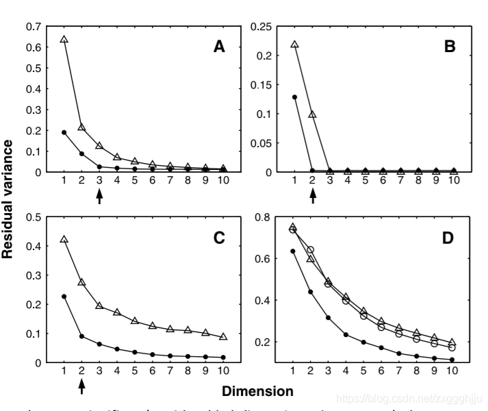
Fig. 2. The residual variance of PCA (open triangles), MDS [open triangles in (A) through ?; open circles in (D)], and Isomap (?lled circles) on four data sets (42). (A) Face images varying in pose and illumination (Fig. 1A). (B) Swiss roll data (Fig. 3). ? Hand images varying in ?nger extension and wrist rotation (20). (D) Handwritten “2”s (Fig.1B). In all cases,residual variance decreases as the dimensionality d is increased. The intrinsic dimensionality of the data can be estimated by looking for the “elbow” at which this curve ceases to decrease signi?cantly with added dimensions. Arrows mark the true or approximate dimensionality, when known. Note the tendency of PCA and MDS to overestimate the dimensionality, in contrast to Isomap.

图2.PCA(空心三角形)、MDS，即(A)至 ( C) 中的空心三角形、(D)中的空心圆和Isoma实心圆对四个数据集（42）的残差。(A)在姿势和照明度上变化的人脸图像（图1 A）；(B)瑞士卷数据（图3）；( C)手部图像，在手指延伸和手腕旋转（20）变化；(D)手写 "2 "（Fig.1B）。在所有情况下，残差随着维度d的增加而减小。数据的内在维度可以通过寻找 "肘部 "来估计，在这个 "肘部 "处，随着维度的增加，曲线不再明显下降。 已知时，箭头标记真实或近似尺寸。请注意，与Isomap相比，PCA和MDS倾向于高估尺寸。

=======================================================================================================

Just as PCA and MDS are guaranteed, given sufficient data, to recover the true structure of linear manifolds, Isomap is guaranteed asymptotically to recover the true dimensionality and geometric structure of a strictly larger class of nonlinear manifolds. Like the Swiss roll, these are manifolds whose intrinsic geometry is that of a convex region of Euclidean space, but whose ambient geometry in the high-dimensional input space may be highly folded, twisted, or curved. For non-Euclidean manifolds, such as a hemisphere or the surface of a doughnut, Isomap still produces a globally optimal lowdimensional Euclidean representation, as measured by Eq. 1.

These guarantees of asymptotic convergence rest on a proof that as the number of data points increases, the graph distances d_G(i,j) provide increasingly better approximations to the intrinsic geodesic distances d_M(i,j), becoming arbitrarily accurate in the limit of infinite data (18, 19). How quickly d_G(i,j) converges to d_M(i,j) depends on certain parameters of the manifold as it lies within the high-dimensional space (radius of curvature and branch separation) and on the density of points. To the extent that a data set presents extreme values of these parameters or deviates from a uniform density, asymptotic convergence still holds in general, but the sample size required to estimate geodesic distance accurately may be impractically large.
就像PCA和MDS在给定足够数据的情况下，可以保证恢复线性流形的真实结构一样，Isomap可以渐进地保证恢复一类严格意义上更大的非线性流形的真实维度和几何结构。就像瑞士卷一样，这些流形的内在几何结构是欧氏空间的凸区域，但其高维输入空间的环境几何结构可能是高度折叠、扭曲或弯曲的。对于非欧几里得表象，如半球形或甜甜圈的表面，Isomap仍能产生全局最优的低维欧几里得表象，由公式1测得。

这些渐近收敛的保证基于以下证明，即随着数据点数量的增加，图形距离d_G(i,j)对固有测地距离d_M(i,j)提供了越来越好的近似值，在无限数据的限制下变得任意精确(18, 19)。d_G(i,j)收敛到d_M(i,j)的速度取决于流形的某些参数，因为它位于高维空间内(曲率半径和分支分离)，并取决于点的密度。如果一个数据集呈现出这些参数的极端值或偏离了均匀的密度，渐进收敛在一般情况下仍然成立，但准确估计测地距离所需的样本量可能不切实际地大。

=======================================================================================================

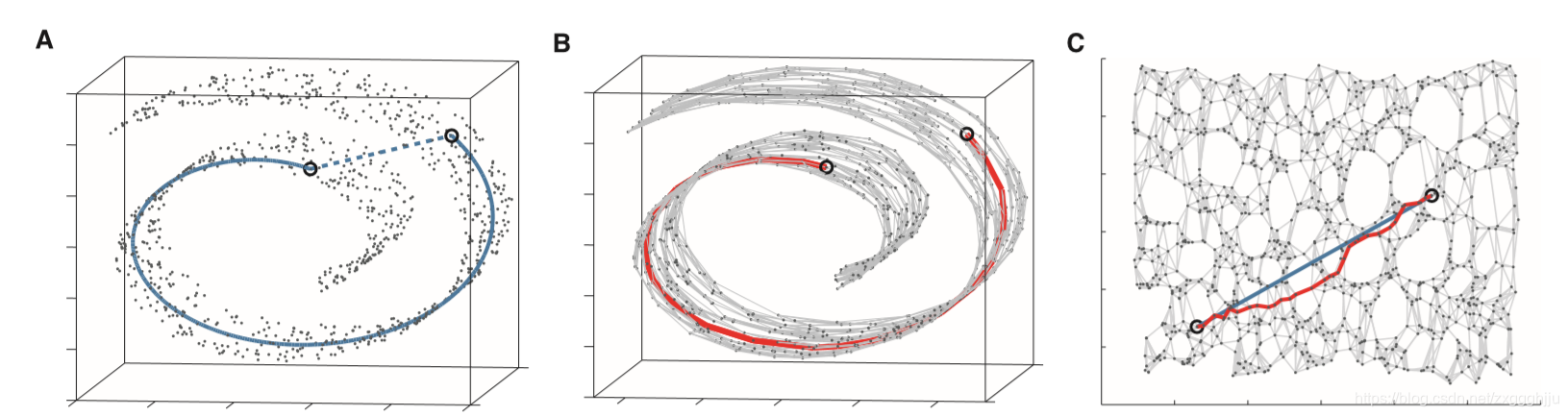
Fig.3.The“Swissroll” dataset,illustrating how Isomap exploits geodesic paths for nonlinear dimensionality reduction.(A) For two arbitrary points (circled) on a nonlinear manifold, their Euclidean distance in the highdimensional input space (length of dashed line) may not accurately re?ect their intrinsic similarity, as measured by geodesic distance along the low-dimensional manifold (length of solid curve). (B) The neighborhood graph G constructed in step one of Isomap (with K=7 and N =1000 data points) allows an approximation (red segments) to the true geodesic path to be computed ef?ciently in step two, as the shortest path in G.( C) The two-dimensional embedding recovered by Isomap in step three, which best preserves the shortest path distances in the neighborhood graph (overlaid). Straight lines in the embedding (blue) now represent simpler and cleaner approximations to the true geodesic paths than do the corresponding graph paths (red).

图3. "瑞士卷"数据集，说明Isomap是如何利用测地路径来降低非线性维度的。 (A) 对于非线性流形上的两个任意带圆圈的点，它们在高维输入空间中的欧氏距离，即虚线的长度可能无法准确地重现它们的内在相似性，这是通过沿低维流形的测地距离，即实曲线的长度测得的。(B)Isomap第一步构建的邻域图G，其K =7，N=1000个数据点，允许在第二步中有效地计算出真正的测地路径的近似值即红色段，作为G中最短的路径。( C)Isomap在第三步中恢复的二维嵌入，它最好的保留邻域图中最短的路径距离(覆盖)。嵌入中的蓝色直线现在比相应的红色图路径更简单、更干净地代表真正的测地路径的近似。

=======================================================================================================

Isomap’s global coordinates provide a simple way to analyze and manipulate highdimensional observations in terms of their intrinsic nonlinear degrees of freedom. For a set of synthetic face images, known to have three degrees of freedom, Isomap correctly detects the dimensionality (Fig. 2A) and separates out the true underlying factors (Fig. 1A). The algorithm also recovers the known low-dimensional structure of a set of noisy real images, generated by a human hand varying in finger extension and wrist rotation (Fig. 2C) (20). Given a more complex data set of handwritten digits, which does not have a clear manifold geometry, Isomap still finds globally meaningful coordinates (Fig. 1B) and nonlinear structure that PCA or MDS do not detect (Fig. 2D). For all three data sets, the natural appearance of linear interpolations between distant points in the low-dimensional coordinate space confirms that Isomap has captured the data’s perceptually relevant structure (Fig. 4).

Isomap的全局坐标提供了一种简单的方法，从其内在的非线性自由度出发，来分析和操作高维度的观测数据。对于一组已知具有三个自由度的合成人脸图像，Isomap正确地检测出尺寸（图2 A），并分离出真正的底层因素（图1 A）。该算法还恢复了已知的一组噪声的真实图像的低维结构，该图像是由一只在手指伸展和手腕旋转中变化的人类手产生的（图2 C）（20）。给定一个更复杂的手写数字数据集，它没有明确的流形几何，Isomap仍然可以找到全局有意义的坐标（图1 B）和非线性结构，而PCA或MDS没有检测到非线性结构（图2D）。对于这三组数据，在低维坐标空间中，远处的点之间自然出现线性插值，证实了Isomap已经捕捉到了数据的感性相关结构（图4）。

=======================================================================================================
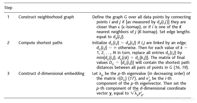
Table1.The Isomap algorithm takes as input the distances d_X(i,j) between all pairs i,j from N datapoints in the high-dimensional input space X, measured either in the standard Euclidean metric (as in Fig. 1A) or in some domain-speci?c metric (as in Fig. 1B). The algorithm outputs coordinate vectors y_i in a d-dimensional Euclidean space Y that (according to Eq. 1) best represent the intrinsic geometry of the data. The only free parameter (ε or K) appears in Step 1.
表1.Isomap算法将高维输入空间X中N个数据点的所有对i,j之间的距离d_X(i,j)作为输入，用标准欧氏度量法，如图1A，或某种域特定度量法，如图1B。该算法在d维欧氏空间Y中输出坐标向量y_i，根据公式1，最能代表数据的内在几何形状。唯一的自由参数ε或K出现在步骤1中。

=======================================================================================================

步骤：
1.构造邻接图 如果[根据d_X(i,j)测量点i和j比ε即ε-Isomap更近，或者如果i是j的K个最近的邻居之一，则通过连接点i和j在所有数据点上定义图G，设置边长等于d_X(i,j)。
2.计算最短路径 如果i,j相连，则初始化d_G(i,j) =d_X(i,j)；否则，初始化d_G(i,j) =∞ 。然后依次对k的每个值1到N，用min{d_G(i,j)，d_G(i,k) +d_G(k,j)}代替所有条目d_G(i,j)。最终值矩阵d_G = {d_G(i,j)}将包含G中所有点对之间的最短路径距离(16，19)。
3.构建d维嵌入 设λ_p为矩阵t(D_G)(17)的第p个特征值(依次递减)， $v^i_p$为p个特征向量的第i个分量。那么设d维坐标矢量y_i的第p个分量等于 $\sqrt{λ_p }v^i_p$

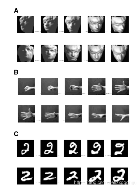
Fig. 4. Interpolations along straight lines in the Isomap coordinate space (analogous to the blue line in Fig. 3C) implement perceptually natural but highly nonlinear “morphs” of the corresponding high-dimensional observations (43) by transforming them approximately along geodesic paths (analogous to the solid curve in Fig. 3A). (A) Interpolations in a three-dimensional embedding of face images (Fig. 1A). (B) Interpolations in a fourdimensional embedding of hand images (20) appear as natural hand movements when viewed in quick succession, even though no such motions occurred in the observed data. ? Interpolations in a six-dimensional embedding of handwritten“2”s(Fig.1B) preserve continuity not only in the visual features of loop and arch articulation, but also in the implied pen trajectories, which are the true degrees of freedom underlying those appearances.

图4.沿着Isomap坐标空间中的直线进行插值，类似于图3C中的蓝线，方法是通过沿测地线近似地变换相应的高维观测值（43），以实现了感知上自然但高度非线性的 “变形”，类似于图3A中的实线。(A) 人脸图像三维嵌入中的插值（图1A）。(B)快速连续观看时，手部图像（20）的四维嵌入中的内插显示为自然的手部运动，即使在观察到的数据中没有发生这样的运动。?手写 "2 "即图1B的六维嵌入中的插值不仅在环形和弓形衔接的视觉特征上保持了连续性，而且在隐含的笔的轨迹上也保持了连续性，这才是这些表象背后的真正自由度。

=======================================================================================================

Previous attempts to extend PCA and MDS to nonlinear data sets fall into two broad classes, each of which suffers from limitations overcome by our approach. Local linear techniques (21–23) are not designed to represent the global structure of a data set within a single coordinate system, as we do in Fig. 1. Nonlinear techniques based on greedy optimization procedures (24–30) attempt to discover global structure, but lack the crucial algorithmic features that Isomap inherits from PCA and MDS: a noniterative, polynomial time procedure with a guarantee of global optimality; for intrinsically Euclidean manifolds, a guarantee of asymptotic convergence to the true structure; and the ability to discover manifolds of arbitrary dimensionality, rather than requiring a fixed d initialized from the beginning or computational resources that increase exponentially in d.

Here we have demonstrated Isomap’s performance on data sets chosen for their visually compelling structures, but the technique may be applied wherever nonlinear geometry complicates the use of PCA or MDS. Isomap complements, and may be combined with, linear extensions of PCA based on higher order statistics, such as independent component analysis (31, 32). It may also lead to a better understanding of how the brain comes to represent the dynamic appearance of objects, where psychophysical studies of apparent motion (33, 34) suggest a central role for geodesic transformations on nonlinear manifolds (35) much like those studied here.

以前尝试将PCA和MDS扩展到非线性数据集的方法分为两大类，每类都受到我们方法克服的局限性的困扰。就像我们在图1中做的那样,局部线性技术(21-23)并不是为了在单一坐标系内表示数据集的全局结构而设计的。基于贪婪优化程序(24-30)的非线性技术试图发现全局结构，但缺乏Isomap从PCA和MDS中继承的关键算法特征：一个非迭代的、多项式时间的程序，并保证全局最优性；对于内在的欧几里德流形，保证了到真实结构的渐近收敛；以及发现任意维度流形的能力，而不需要从开始就初始化的固定d或在d中呈指数增长的计算资源。

在这里，我们已经展示了Isomap在为其视觉上引人注目的结构选择的数据集上的性能，但该技术可以应用在任何非线性几何形状复杂的PCA或MDS的使用。Isomap是对基于高阶统计学的PCA线性扩展的补充，也可以与之结合，如独立成分分析(31, 32)。它也可能导致人们更好地理解大脑如何来表示对象的动态外观，其中视运动的心理物理学研究（33，34）提出了非线性流形上的测地线变换（35）的中心作用，很像那些在这里研究。

=======================================================================================================
References and Notes

1. M. P. Young, S. Yamane, Science 256, 1327 (1992).
2. R. N. Shepard, Science 210, 390 (1980).
3. M. Turk, A. Pentland, J. Cogn. Neurosci. 3, 71 (1991).
4. H. Murase, S. K. Nayar, Int. J. Comp. Vision 14,5 (1995).
5. J. W. McClurkin, L. M. Optican, B. J. Richmond, T. J. Gawne, Science 253, 675 (1991).
6. J. L. Elman, D. Zipser, J. Acoust. Soc. Am. 83, 1615 (1988).
7. W. Klein, R. Plomp, L. C. W. Pols, J. Acoust. Soc. Am. 48, 999 (1970).
8. E.Bizzi,F.A.Mussa-Ivaldi,S.Giszter,Science253,287 (1991).
9. T. D. Sanger, Adv. Neural Info. Proc. Syst. 7, 1023 (1995).
10. J. W. Hurrell, Science 269, 676 (1995).
11. C. A. L. Bailer-Jones, M. Irwin, T. von Hippel, Mon. Not. R. Astron. Soc. 298, 361 (1997).
12. P. Menozzi, A. Piazza, L. Cavalli-Sforza, Science 201, 786 (1978).
13. K. V. Mardia, J. T. Kent, J. M. Bibby, Multivariate Analysis, (Academic Press, London, 1979).
14. A. H. Monahan, J. Clim., in press.
15. The scale-invariant K parameter is typically easier to set than ε, but may yield misleading results when thlocal dimensionality varies across the data set. When available, additional constraints such as the temporal ordering of observations may also help to determine neighbors. In earlier work (36) we explored a more complex method (37), which required an order of magnitude more data and did not support the theoretical performance guarantees we provide here for ε- and K-Isomap.
16. This procedure, known as Floyd’s algorithm, requires O(N³) operations. More ef?cient algorithms exploiting the sparse structure of the neighborhood graph can be found in (38).
17. The operator t is de?ned by τ (D)= -HSH/2, where S is the matrix of squared distances ${S_{ij} = D_{ij}^ 2}$, and H is the “centering matrix” {H_ij = δ_ij -1/N}(13).
18. Our proof works by showing that for a suf?ciently highdensity( α) of data points,we can always choose a neighborhood size (ε or K) large enough that the graph will (with high probability) have a path not much longer than the true geodesic, but small enough to prevent edges that “short circuit” the true geometry of the manifold. More precisely, given arbitrarily small values of λ₁,λ₂, and μ, we can guarantee that with probability at least 1- μ, estimates of the form
    $(1-λ_1)d_M(i,j)\leqslant d_G(i,j)\leqslant(1+λ_2)d_M(i,j)$
    will hold uniformly over all pairs of data points i,j.For ε-Isomap, we require
    $ε\leqslant (2/π)r_0\sqrt{24λ_1}$ ε <s₀,
    $α>[log(V/μη_d(λ_2\epsilon/16)^d)]/\eta _d(\lambda _2\epsilon/8)^d$
    where r₀ is the minimal radius of curvature of the manifold M as embedded in the input space X, s₀ is the minimal branch separation of M in X, V is the (d-dimensional)volume of M,and (ignoringboundary effects) η_d is the volume of the unit ball in Euclidean d-space. For K-Isomap, we let ε be as above and ?x the ratio (K +1)/α=η_d(ε/2)^d/2. We then require
    $e^{-(k+1)/4}\leqslant \mu \eta _d(\varepsilon /4)^d/4V$
    $(e/4)^{(k+1)/2}\leqslant \mu \eta _d(\varepsilon /8)^d/16V$
    $\alpha >[4log(8V/\mu \eta _d(\lambda _2\varepsilon /32\Pi )^d)]/\eta _d(\lambda _2\varepsilon /16\Pi )^d$
    The exact content of these conditions—but not their general form—depends on the particular technical assumptions we adopt. For details and extensions to nonuniform densities, intrinsic curvature, and boundary effects, see http://isomap.stanford.edu.
19. In practice, for ?nite data sets, d_G(i,j) may fail to approximate d_M(i,j) for a small fraction of points that are disconnected from the giant component of the neighborhood graph G. These outliers are easily detected as having in?nite graph distances from the majority of other points and can be deleted from further analysis.
20. The Isomap embedding of the hand images is available at Science Online at www.sciencemag.org/cgi/content/full/290/5500/2319/DC1. For additional material and computer code, see http://isomap. stanford.edu.
21. R. Basri, D. Roth, D. Jacobs, Proceedings of the IEEE Conference on Computer Vision and Pattern Recognition (1998), pp. 414–420.
22. C. Bregler, S. M. Omohundro, Adv. Neural Info. Proc. Syst. 7, 973 (1995).
23. G. E. Hinton, M. Revow, P. Dayan, Adv. Neural Info. Proc. Syst. 7, 1015 (1995).
24. R. Durbin, D. Willshaw, Nature 326, 689 (1987).
25. T. Kohonen, Self-Organisation and Associative Memory (Springer-Verlag, Berlin, ed. 2, 1988), pp. 119– 157.
26. T. Hastie, W. Stuetzle, J. Am. Stat. Assoc. 84, 502 (1989).
27. M. A. Kramer, AIChE J. 37, 233 (1991).
28. D. DeMers, G. Cottrell, Adv. Neural Info. Proc. Syst. 5, 580 (1993).
29. R. Hecht-Nielsen, Science 269, 1860 (1995).
30. C. M. Bishop, M. Svens?en, C. K. I. Williams, Neural Comp. 10, 215 (1998).
31. P. Comon, Signal Proc. 36, 287 (1994).
32. A. J. Bell, T. J. Sejnowski, Neural Comp. 7, 1129 (1995).
33. R. N. Shepard, S. A. Judd, Science 191, 952 (1976).
34. M. Shiffrar, J. J. Freyd, Psychol. Science 1, 257 (1990).
35. R. N. Shepard, Psychon. Bull. Rev. 1, 2 (1994).
36. J. B. Tenenbaum, Adv. Neural Info. Proc. Syst. 10, 682 (1998).
37. T.Martinetz,K.Schulten,NeuralNetw.7,507(1994).
38. V. Kumar, A. Grama, A. Gupta, G. Karypis, Introduction to Parallel Computing: Design and Analysis of Algorithms (Benjamin / Cummings, Redwood City, CA, 1994), pp. 257–297.
39. D. Beymer, T. Poggio, Science 272, 1905 (1996).
40. Available at www.research.att.com/;yann/ocr/mnist.
41. P. Y. Simard, Y. LeCun, J. Denker, Adv. Neural Info. Proc. Syst. 5, 50 (1993).
42. In order to evaluate the ?ts of PCA, MDS, and Isomap on comparable grounds, we use the residual variance
    1–R²(D _M, D_Y). D_Y is the matrix of Euclidean distances in the low-dimensional embedding recovered by each algorithm. D _M is each algorithm’s best estimate of the intrinsic manifold distances: for Isomap, this is the graph distance matrix D_G; for PCA and MDS, it is the Euclidean input-space distance matrix D_X (except with the handwritten “2”s, where MDS uses the tangent distance). R is the standard linear correlation coef?cient, taken over all entries of D _M and D_Y.
43. In each sequence shown, the three intermediate images are those closest to the points 1/4, 1/2, and 3/4 of the way between the given endpoints.We can also synthesize an explicit mapping from input space X to the low-dimensional embedding Y, or vice versa, using the coordinates of corresponding points {xi, yi} in both spaces provided by Isomap together with standard supervised learning techniques (39).
44. Supported by the Mitsubishi Electric Research Laboratories, the Schlumberger Foundation, the NSF (DBS-9021648), and the DARPA Human ID program. We thank Y. LeCun for making available the MNIST database and S.RoweisandL.Saulforsharingrelated unpublished work. For many helpful discussions, we thank G. Carlsson, H. Farid, W. Freeman, T. Grif?ths, R. Lehrer, S. Mahajan, D. Reich, W. Richards, J. M. Tenenbaum, Y. Weiss, and especially M. Bernstein.

10 August 2000; accepted 21 November 2000