【论文翻译】Task Difficulty Aware Parameter Allocation Regularization for Lifelong Learning

Task Difficulty Aware Parameter Allocation & Regularization for Lifelong Learning

面向终身学习的任务难度感知参数分配与正则化

摘要

Recently, many parameter regularization or allocation methods have been proposed to overcome catastrophic forgetting in lifelong learning. However, they treat all tasks in a sequence equally and solve them uniformly, ignoring differences in the learning difficulty of different tasks. This results in significant forgetting in parameter regularization when learning a new task very different from learned tasks, and also leads to unnecessary parameter overhead in parameter allocation when learning simple tasks. Instead, a natural idea is allowing the model adaptively select an appropriate strategy from parameter allocation and parameter regularization according to the learning difficulty of each task. To this end, we propose a new lifelong learning framework named Parameter Allocation & Regularization (PAR) based on two core concepts: task group and expert. A task group consists of multiple relevant tasks that have been learned by the same expert. A new task is easy for an expert if it is relevant to the corresponding task group, and we reuse the expert for it by parameter regularization. Conversely, a new task is difficult for the model if all task groups are not relevant to it, then we treat it as a new task group and allocate a new expert for it. To measure the relevance between tasks, we propose a divergence estimation method via Nearest-Prototype distance. To reduce the parameter overhead of experts, we propose a time efficient relevance-aware sampling-based architecture search strategy. Experimental results on 6 benchmarks show that, compared with SOTAs, our method is scalable and significantly reduces the model redundancy while improving the model performance. Further, qualitative analysis shows that the task relevance obtained by our method is reasonable.

近年来，人们提出了许多参数正则化或分配方法来克服终身学习中的灾难性遗忘。然而，他们将所有任务一视同仁，统一解决，忽略了不同任务学习难度的差异。这会导致在学习与已学习任务截然不同的新任务时，参数正则化的显著遗忘，并且在学习简单任务时，会导致参数分配中不必要的参数开销。相反，一个自然的想法是允许模型根据每个任务的学习难度，从参数分配和参数正则化中自适应地选择合适的策略。为此，我们提出了一个新的终身学习框架，名为参数分配与正则化（PAR），该框架基于两个核心概念：任务组和专家。任务组由同一专家学习的多个相关任务组成。如果一个新任务与相应的任务组相关，那么它对专家来说很容易，我们通过参数正则化重用专家。相反，如果所有的任务组都与模型无关，那么新的任务对模型来说是困难的，那么我们将其视为一个新的任务组，并为其分配新的专家。为了度量任务之间的相关性，我们提出了一种基于最近原型距离的发散度估计方法。为了减少专家的参数开销，我们提出了一种基于时间效率的相关性感知采样架构搜索策略。在6个基准测试上的实验结果表明，与SOTA相比，该方法具有可扩展性，在提高模型性能的同时显著降低了模型冗余。此外，定性分析表明，该方法得到的任务相关性是合理的。

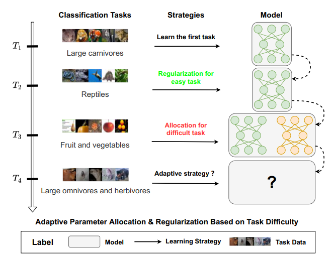
Figure 1: In lifelong learning, the learning difficulty of each task is different and depends not only on itself but also on tasks the model has learned before. A natural idea is to allow the model adaptively select an appropriate strategy to handle each task according to its learning difficulty. For example, task?2 (Reptiles) is easy for the model that has learned task?1 (Large carnivores) and parameter regularization is sufficient to adapt to it. On the contrary, task ?3 (fruit and vegetables) is still difficult for the model that has learned tasks ?1 and ?2 and parameter allocation is necessary for it.    在终身学习中，每个任务的学习难度是不同的，不仅取决于任务本身，还取决于模型以前学习过的任务。一个自然的想法是允许模型根据学习难度自适应地选择适当的策略来处理每个任务。例如，任务?2（爬行动物）对于学习过任务的模型来说很容易?1（大型食肉动物）和参数正则化足以适应它。相反，任务?3（水果和蔬菜）对于学习过任务的模型来说仍然很难?1和?2.参数分配是必要的。 

介绍

Recently, the lifelong learning[11] ability of neural networks, i.e.,learning continuously from a continuous sequence of tasks, has been extensively studied. It is natural for human beings to constantly learn and accumulate knowledge from tasks and then use it to facilitate future learning. However, existing classical models [17, 22] suffer catastrophic forgetting [15], in which the model’s performance on learned tasks deteriorates rapidly after learning a new one.

最近，神经网络的终身学习能力[11]得到了广泛的研究，即从一系列连续的任务中不断学习。人类自然会不断地从任务中学习和积累知识，然后利用这些知识促进未来的学习。然而，现有的经典模型[17,22]遭受了灾难性遗忘[15]，在这种情况下，模型在学习新任务后，学习任务的性能会迅速降低。

To overcome the catastrophic forgetting, many lifelong learning methods have been proposed (more details in Section 2). Parameter regularization methods [12, 20, 23, 25, 27, 29, 32] try to alleviate forgetting by introducing a regularization term in the loss function and perform well when the new task does not differ much from learned tasks. Parameter allocation methods based on static models [9, 19, 36, 42] and dynamic models [2, 24, 28, 30, 34, 35, 40, 44, 45, 47, 50, 53] allocate different parameters to different tasks and can adapt to new tasks that are quite different from the tasks learned before.

为了克服灾难性遗忘，人们提出了许多终身学习方法（更多细节见第2节）。参数正则化方法[12,20,23,25,27,29,32]试图通过在损失函数中引入正则化项来缓解遗忘，并且在新任务与学习任务没有太大差异时表现良好。基于静态模型[9,19,36,42]和动态模型[2,24,28,30,34,35,40,44,45,47, 50,53]的参数分配方法为不同的任务分配不同的参数，并且能够适应与之前学习的任务有很大不同的新任务。

However, they treat all tasks in a sequence equally and try to solve them uniformly, and ignore differences in the learning difficulty of different tasks in the sequence. This results in significant forgetting of parameter regularization methods when learning a new task that is very different from learned tasks, and also leads to unnecessary parameter overhead of parameter allocation methods when learning some simple tasks.

然而，他们平等地对待序列中的所有任务，并试图统一解决它们，而忽略序列中不同任务学习难度的差异。这导致在学习与学习任务截然不同的新任务时，参数正则化方法被显著遗忘，并且在学习一些简单任务时，参数分配方法也会产生不必要的参数开销。

Instead, a natural idea is to allow the model to adaptively select an appropriate strategy from parameter allocation and parameter regularization for each task according to its learning difficulty. In this paper, we propose a new lifelong learning framework named Parameter Allocation & Regularization (PAR) based on two core concepts: task group and expert, where a task group consists of multiple relevant tasks that have been learned by the same expert. Based on the above two concepts, we adaptively tackle different tasks with different strategies according to their difficulty. Specifically, a new task is easy for an expert if it is relevant to the corresponding task group of the expert, and we reuse the expert for it by parameter regularization. Conversely, a new task is difficult for the model if all task groups are not relevant to it, then we treat it as a new task group and allocate a new expert for it.

相反，一个自然的想法是允许模型根据每个任务的学习难度，从参数分配和参数正则化中自适应地选择合适的策略。本文基于任务组和专家两个核心概念，提出了一个新的终身学习框架——参数分配与正则化（PAR），其中任务组由同一专家学习的多个相关任务组成。基于以上两个概念，我们根据不同任务的难度，采用不同的策略自适应地处理不同的任务。具体来说，如果一个新任务与专家的相应任务组相关，那么它对专家来说是容易的，并且我们通过参数正则化为它重新使用专家。相反，如果所有的任务组都与模型无关，那么新的任务对模型来说是困难的，那么我们将其视为一个新的任务组，并为其分配新的专家。

The main challenges of our method are (1) how to measure the relevance between tasks and (2) how to control the parameter overhead associated with parameter allocation. For challenge (1), we measure the relevance between two tasks by the distance between their feature distributions. Since only the data of the current task is available in the lifelong learning scenario, we cannot measure the distance between the feature distributions of two tasks directly by similarity functions that requires data from both tasks, such as cosine, KL divergence or ?? norm. To solve this problem, we propose a divergence estimation method based on prototype distance. For challenge (2), we control the overall parameter overhead by reducing the number of parameters per expert model. Specifically, we search the appropriate model architecture for each expert to make sure it is compact enough. Because lifelong learning algorithms need to deal with a sequence of tasks, in this scenario, the low time and memory efficiency of architectural search algorithms is a great obstacle. To solve this problem, we propose a relevanceaware sampling-based architecture search strategy, which is time and memory efficient.

我们的方法面临的主要挑战是：（1）如何测量任务之间的相关性；（2）如何控制与参数分配相关的参数开销。对于挑战（1），我们通过两个任务的特征分布之间的距离来衡量它们之间的相关性。由于终身学习场景中只有当前任务的数据可用，因此我们无法通过需要两个任务数据的相似性函数（如余弦、KL散度或方差）直接测量两个任务的特征分布之间的距离?? 标准。为了解决这个问题，我们提出了一种基于原型距离的散度估计方法。对于挑战（2），我们通过减少每个专家模型的参数数量来控制总体参数开销。具体来说，我们为每位专家搜索合适的模型体系结构，以确保其足够紧凑。由于终身学习算法需要处理一系列任务，在这种情况下，体系结构搜索算法的低时间和内存效率是一个很大的障碍。为了解决这个问题，我们提出了一种基于相关软件采样的架构搜索策略，该策略既节省时间又节省内存。

Our main contributions are summarized as follows:
(1) To adaptively select an appropriate strategy from parameter allocation and parameter regularization for each task according to its learning difficulty, we propose a new lifelong learning framework named Parameter Allocation & Regularization (PAR) based on two core concepts: task group and expert. With these two concepts, our method can flexibly reuse an existing expert or assign a new expert for a new tasks according to the relevance between the new task
and existing task groups.
(2) To measure the relevance between tasks and control the overall parameter overhead, we propose a divergence estimation method based on prototype distance and a relevance-aware sampling-based architecture search strategy.
(3) Experimental results on multiple benchmarks, including CTrL, Mixed CIFAR100 and F-CelebA, CIFAR10-5, CIFAR100-10, CIFAR100-20 and MiniImageNet-20, show that our method is scalable and significantly reduces the redundancy of the model while improving the performance of the model. Exhaustive ablation studies show that each component in our method is valid. Further, analyses of divergence estimation show that task relevance obtained by our method is reasonable.

我们的主要贡献总结如下：
（1） 为了根据每个任务的学习难度，从参数分配和参数正则化中自适应地选择合适的策略，我们基于任务组和专家两个核心概念，提出了一个新的终身学习框架参数分配与正则化（PAR）。有了这两个概念，我们的方法可以灵活地重用现有专家或根据新任务之间的相关性为新任务指派新专家
以及现有的任务组。
（2） 为了测量任务之间的相关性并控制总体参数开销，我们提出了一种基于原型距离的散度估计方法和一种基于相关性感知采样的架构搜索策略。
（3） 在CTrL、Mixed CIFAR100和F-CelebA、CIFAR10-5、CIFAR100-10、CIFAR100-20和MiniImageNet-20等多个基准上的实验结果表明，我们的方法具有可扩展性，显著减少了模型的冗余，同时提高了模型的性能。详尽的烧蚀研究表明，我们方法中的每个成分都是有效的。此外，对散度估计的分析表明，该方法得到的任务相关性是合理的。

2  相关工作

2.1 Lifelong Learning

Many methods have been proposed to overcome catastrophic forgetting. Replay methods try to replay samples of previous tasks when learning a new task from an episodic memory [37, 46] or a generative memory [3, 33, 43]. Parameter regularization methods [12, 20, 23, 25, 27, 29, 32], including prior-focused regularization and data-focused regularization, try to alleviate forgetting by introducing a regularization term in the loss function of new tasks. Parameter allocation methods based on the static model [9, 19, 36, 42] or dynamic model [2, 24, 28, 30, 34, 35, 40, 44, 45, 47, 50, 53] overcome catastrophic forgetting by allocating different parameters to different tasks. In addition, [18, 39] propose to directly learn a model that performs well in the lifelong learning scenario by meta-learning methods. [10, 51] focus on the problem of data imbalance during lifelong learning. [31] focuses on the effect of training regimes in lifelong learning. Further, the problem of lifelong learning is studied in richer scenarios [4, 16]

人们提出了许多克服灾难性遗忘的方法。重放方法尝试在从情景记忆[37,46]或生成性记忆[3,33,43]学习新任务时重放先前任务的样本。参数正则化方法[12,20,23,25,27,29,32]，包括先验聚焦正则化和数据聚焦正则化，试图通过在新任务的损失函数中引入正则化项来缓解遗忘。基于静态模型[9,19,36,42]或动态模型[2,24,28,30,34,35,40,44,45,47,50,53]的参数分配方法通过为不同的任务分配不同的参数来克服灾难性遗忘。此外，[18,39]建议通过元学习方法直接学习在终身学习场景中表现良好的模型。[10,51]关注终身学习期间的数据不平衡问题。[31]关注培训制度对终身学习的影响。此外，终身学习的问题在更丰富的场景中进行了研究[4,16]。

2.2 Cell-based NAS

Neural architecture search (NAS) [14, 38] aims to search for efficient neural network architectures from a predefined search space in a data-driven manner. To reduce the size of the search space, cellbased NAS methods [26, 54, 55] try to search for a cell architecture from a predefined cell search space, where a cell is defined as a tiny convolutional network mapping an ? ×? ×? tensor to another ? ′×? ′×? ′. The final model consists of a predefined number of stacked cells. The cell in NAS is similar to the concept of residual block in the residual network but with a more complex architecture, which is a directed acyclic graph (DAG). Since operations in the search space are parameter efficient, the architectures obtained by NAS are usually more compact than hand-crafted architectures. In this paper, we adopt cell-based NAS to search compact cell architectures for experts, which reduces the parameter overhead in the parameter allocation phase.

神经架构搜索（NAS）[14,38]旨在以数据驱动的方式从预定义的搜索空间中搜索高效的神经网络架构。为了减少搜索空间的大小，基于单元的NAS方法[26、54、55]尝试从预定义的单元搜索空间中搜索单元架构，其中单元被定义为映射? ×? ×? 张量? ′×? ′×? ′. 最终的模型由预定义数量的堆叠单元组成。NAS中的单元类似于剩余网络中剩余块的概念，但具有更复杂的体系结构，即有向无环图（DAG）。由于搜索空间中的操作具有参数效率，NAS获得的体系结构通常比手工构建的体系结构更紧凑。在本文中，我们采用基于小区的NAS为专家搜索紧凑的小区体系结构，这减少了参数分配阶段的参数开销。

2.3 Comparison and Discussion

Methods with task relevance. ExpertGate [2] and CAT [19] also consider task relatedness but with a different focus than ours. (i) The calculation of task relevance in our method is different from them; (ii) We focus on the relevance between the new task and each existing task groups, but ExpertGate focus on the relatedness between the new task and each previous task; (iii) ExpertGate assigns a dedicated expert to each task, but each expert in our method are shared by tasks in the same group; CAT [19] defines the task similarity by the positive knowledge transfer. It focuses on selectively transferring the knowledge from similar previous tasks and dealing with forgetting between dissimilar tasks by hard attention.

具有任务相关性的方法。 ExpertGate〔2〕和CAT〔19〕也考虑了任务关联性，但与我们的关注点不同。（i） 我们的方法对任务相关性的计算不同于它们；（ii）我们关注新任务与每个现有任务组之间的相关性，而ExpertGate关注新任务与每个先前任务之间的相关性；（iii）ExpertGate为每项任务指定一位专门的专家，但我们方法中的每一位专家都由同一组中的任务共享；CAT[19]通过正向知识转移定义了任务相似性。它侧重于有选择地转移以前类似任务中的知识，并通过硬注意处理不同任务之间的遗忘。

Methods with NAS. [9, 36] try to search a sub-model for each task with NAS methods. [24, 47, 52] adopt NAS approaches to select the appropriate model expansion strategy for each task and face the high GPU memory, parameter, and time overhead. Different from the above methods, we adopt the cell-based NAS to search a compact architecture for each expert with the lower GPU memory and parameter overhead. We also adopt a cell sharing strategy among experts to reduce the time overhead.

使用NAS的方法。[9,36]尝试使用NAS方法搜索每个任务的子模型。[24、47、52]采用NAS方法为每项任务选择合适的型号扩展策略，并面临高GPU内存、参数和时间开销。与上述方法不同，我们采用基于单元的NAS为每个专家寻找一个紧凑的体系结构，具有较低的GPU内存和参数开销。我们还采用了专家间的单元共享策略，以减少时间开销。

3 方法

3.1 Problem Formulation and Method Overview

There are two scenarios for lifelong learning: class incremental learning and task incremental learning. In this paper, we focus on the task incremental scenario, where the task id of each sample is available during both the training and inference. Specifically, given a sequence of N tasks, denoted as T = {?1, . . . ,??, . . . ,?? }, a model needs to learn them one by one. Each task ?? has a training dataset, ?? ????? = {(???,??? );? = 1, . . . , ?? ?????}, where ??? is the true label and ?? ????? is the number of training examples. Similarly, we can denote the validation and test dataset of task ?? as ?? ????? and ????? ? .

终身学习有两种场景：类增量学习和任务增量学习。在本文中，我们关注任务增量场景，其中每个样本的任务id在训练和推理期间都可用。具体来说，给定N个任务的序列，表示为T = {?1, . . . ,??, . . . ,?? }, 模型需要一个接一个地学习。每项任务?? 有一个训练数据集，, 其中是真正的标签和是训练示例的数量。同样，我们可以表示任务的验证和测试数据集?? 如 .

The key idea in our method is to allow the model to adaptively select an appropriate strategy from parameter allocation and parameter regularization according to the learning difficulty of each new task to overcome the catastrophic forgetting. Our method consists of two core concepts: task group and expert. A task group consists of multiple relevant tasks that have been learned by the same expert. Based on above concepts, we can measure the learning difficulty of each task according to the relevance between the tasks and existing task groups. A new task is easy for an expert if it is relevant to the corresponding task group of the expert, and we reuse the expert for it by parameter regularization. Conversely, a new task is difficult for the model if all task groups are not relevant to it, then we treat it as a new task group and allocate a new expert for it.

该方法的核心思想是让模型根据每个新任务的学习难度，从参数分配和参数正则化中自适应地选择合适的策略，以克服灾难性遗忘。我们的方法由两个核心概念组成：任务组和专家。任务组由同一专家学习的多个相关任务组成。基于上述概念，我们可以根据任务与现有任务组之间的相关性来衡量每个任务的学习难度。如果新任务与专家的相应任务组相关，则专家可以轻松完成该任务，并通过参数正则化重新使用专家。相反，如果所有的任务组都与模型无关，那么新的任务对模型来说是困难的，那么我们将其视为一个新的任务组，并为其分配新的专家。

Specifically, for each new task, we measure the relevance between the new task and existing task groups by a divergence estimation method based on prototype distance and select an appropriate strategy from parameter regularization and parameter allocation according to the relevance (Sect. 3.2). For parameter regularization, we allow the new task reuse the expert of the most relevance task group. Depending on the scale of the new task and previous learned tasks, knowledge distillation and parameter freezing are used to mitigate forgetting, respectively. For parameter allocation, we build a new task group for the new task and allocate a new expert. To reduce the parameter overhead of experts, we propose a relevanceaware sampling-based architecture search strategy, which is time efficient and ensures the architecture of each expert is compact. Each expert in our method is stacked with multiple modules of the same architecture. Following the common practice in NAS, we call such a module a cell. Therefore, searching the appropriate architecture for the expert is equivalent to searching the appropriate cell.

具体来说，对于每个新任务，我们通过基于原型距离的发散度估计方法测量新任务和现有任务组之间的相关性，并根据相关性从参数正则化和参数分配中选择合适的策略（第3.2节）。对于参数正则化，我们允许新任务重用最相关任务组的专家。根据新任务和先前学习任务的规模，分别使用知识提取和参数冻结来缓解遗忘。对于参数分配，我们为新任务建立一个新的任务组，并分配一个新的专家。为了减少专家的参数开销，我们提出了一种基于相关软件采样的架构搜索策略，该策略既节省时间，又保证了每个专家的架构紧凑。我们方法中的每个专家都由相同体系结构的多个模块组成。按照NAS中的常见做法，我们将这样的模块称为单元。因此，为专家搜索合适的体系结构相当于搜索合适的单元。

3.2 Task Relevance and Strategy

In our method, we use the relevance between the new task and existing task groups to measure the task learning difficulty. Specifically, we adopt the distance between the distribution of data of two tasks as the relevance score between two tasks. However, in the lifelong learning scenario, only the data of the current task is available. So we cannot measure the distance directly by similarity functions that requires data from both tasks, such as cosine, KL divergence or ?? norm. To solve this problem, we propose a divergence estimation method via prototype distance, which is inspired by the divergence estimation via ?-Nearest-Neighbor distances [49].

在我们的方法中，我们使用新任务和现有任务组之间的相关性来测量任务学习难度。具体来说，我们采用两个任务的数据分布之间的距离作为两个任务之间的相关性得分。然而，在终身学习场景中，只有当前任务的数据可用。因此，我们无法通过相似性函数直接测量距离，而相似性函数需要来自两个任务的数据，例如余弦、KL散度或距离?? 标准。为了解决这个问题，我们提出了一种基于原型距离的散度估计方法，该方法受到了基于原型距离的散度估计的启发?-最近邻距离[49]。

Before getting into the details, we denote the new task as ?? and the set of existing task groups as G. Then, the ?-th task group is denoted as G? and the ?-th task in group G? is denoted as ???. The details of relevance calculation and task difficulty aware strategy is as follows:

在讨论细节之前，我们将新任务表示为?? ，现有任务组的集合为G。然后第?个任务组被表示为G? ，G?的第?个任务表示为. 相关性计算和任务难度感知策略的细节如下：

Robust data representation. To enhance the stability of relevance calculation, we use a extractor, i.e. ResNet18 pre-trained on ImageNet, to generate a robust feature ??? for each image ??? . Note that the pre-trained extractor is only used for relevance calculation and does not affect the learning of tasks. The extra parameters introduced by this extractor are fixed and do not increase with the number of tasks, so it does not affect the scalability of our method .

稳健的数据表示。为了增强相关性计算的稳定性，我们使用了一个提取器，即在ImageNet上预训练的ResNet18，来生成一个健壮的特征对于每个图像 . 请注意，预先训练的提取器仅用于相关性计算，不影响任务的学习。这个提取器引入的额外参数是固定的，不会随着任务数量的增加而增加，因此它不会影响我们方法的可伸缩性。

Divergence estimation via ?-Nearest-Neighbor distances. Suppose that the robust features ?? = {?1?, . . . , ??? } and ? ? = {?1?, . . . , ??? } of two task ?? and ?? , where ? and ? are the number of samples, are drawn independently from distributions ?? and ?? respectively, [49] shows that KL divergence between two distributions can be estimated as follows:

发散度估计?-最近邻距离。假设健壮的特征两个任务中的一个?? 和?? , 其中? 和? 是独立于分布提取的样本数?? 和?? [49]分别表明，两个分布之间的KL差异可以估计如下：

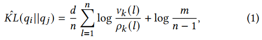
where ?? (?) is the Euclidean distance from ??? to its?-NN in {??? }?≠? , ?? (?) is the distance from ??? to its ?-NN in ? ? , and ? is the dimension of features. Readers can refer to [49] for more details such as convergence analysis. However, the calculation of formula (1) involves data of two tasks, which is not consistent with the lifelong learning scenario. We adapt formula (1) into lifelong learning by replace ?-NN distances with Nearest-Prototype distances.

其中?? (?) 是的欧几里得距离到它中的?-NN  , ?? (?) 距离是 到它 ? ?中的?-NN , ? 是特征的维度。读者可以参考[49]了解更多细节，如收敛分析。然而，公式（1）的计算涉及两项任务的数据，这与终身学习情景不一致。我们通过替换将公式（1）调整为终身学习?-NN距离与最近的原型距离。

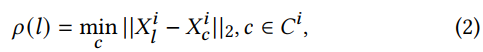
Divergence estimation via Nearest-Prototype distances. For each class ? of task ??, we maintain a prototype feature ???, which is the mean of features of samples that belong to this class. Suppose the set of classes in task ?? is ??, then the Nearest-Prototype distance of ?? ? to ?? is defined as follows:

通过最近的原型距离进行散度估计。每个类别? 任务范围??, 我们维护一个原型功能, 这是属于这个类别的样本特征的平均值。假设任务中有一组类?? 是??, 那么最接近的原型距离到?? 定义如下：

where || · || is the Euclidean distance. Similarly, we the NearestPrototype distance of ??? to ? ? is denoted as

其中| |·| |是欧几里得距离。同样地，我们也得到了 到? ? 表示为

where ?? is the set of classes in task ?? . By replacing ?-Nearestdistances in formula (1) with Nearest-Prototype distances, we estimate KL divergence between two distributions as follows: 

其中?? 是任务中的一组类?? . 通过替换?-在公式（1）中，利用最近的原型距离，我们估计两个分布之间的KL散度，如下所示：

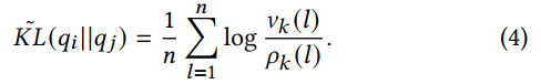
For simplicity, we omit some constant terms, because we are only concerned with the relative magnitude of KL divergence.

为了简单起见，我们省略了一些常数项，因为我们只关心KL散度的相对大小。

Task distance. We directly use the divergence between two task ?? and ?? estimated by formula (4) as the distance between them.

任务距离。我们直接使用两个任务之间的差异?? 和?? 通过公式（4）估算为它们之间的距离。

The more relevant the two tasks are, the smaller the task distance is; otherwise, the larger the task distance is. Then, the distance between a task ?? and a task group G? is calculated as follows:

两个任务的相关性越大，任务距离越小；否则，任务距离越大。然后，任务之间的距离?? 和一个工作组G? 计算如下：

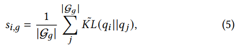
 where ?? and ?? represent feature distributions of task ?? and the ?-th task in group G?.

其中?? 和?? 表示任务的特征分布?? 还有第?组的第四项任务G?.

Adaptive learning strategy for new task ?? . We denote the task group most relevant to the new task ?? , i.e. the task group with the lowest task distance with task ?? , as G?? and the corresponding relevance score is denoted as. To select a strategy for task ?? , we introduce a hyper-parameter ?. When ≤ ?, the new task is sufficiently relevant to the task group G??. Then, we add the new task into group G?? and reuse the expert of this group, denoted as ?? ?, for the new task by parameter regularization (Sect. 3.3). On the contrary, when > ?, the new task is not relevant to all existing task groups. Then, we create a new task group for it and adopt parameter allocation to learn it (Sect. 3.4).

适应新任务的学习策略?? . 我们表示与新任务最相关的任务组?? , 也就是与任务距离最小的任务组?? , 作为G?? 相应的相关性得分表示为. 为任务选择策略?? , 我们引入了一个超参数?. 什么时候 ≤ ?, 新任务与任务组G有足够的相关性??. 然后，我们将新任务添加到G组中?? 重复使用该组的专家，表示为?? ?, 对于通过参数正则化的新任务（第3.3节）。相反，当 > ?, 新任务与所有现有任务组无关。然后，我们为它创建一个新的任务组，并采用参数分配来学习它（第3.4节）。

Failure of task distance. When the number of samples in a task is very small, such as only several samples, the task distance obtained by our method may not be accurate enough. The reason is that bias and variance in formula (1) vanish as sample sizes increase [49]. To avoid the above problem, we directly use parameter regularization for tasks with small data, regardless of task distance.

任务距离失败。当一个任务中的样本数很小时，例如只有几个样本，我们的方法得到的任务距离可能不够精确。原因是公式（1）中的偏差和方差随着样本量的增加而消失[49]。为了避免上述问题，我们直接对小数据任务使用参数正则化，而不考虑任务距离。

 3.3 Parameter Regularization

When new task ?? is easy for the expert ???, we reuse the expert to learn the new task by parameter regularization.

新任务何时开始?? 这对专家来说很容易???, 我们通过参数正则化重用专家学习新任务。

Inspired by LwF [25], we adopt a data-focused parameter regularization method based on knowledge distillation. Specifically, the loss function consists of two parts: training loss L??? and distillation loss L??? . The training loss, i.e. the cross-entropy for classification, encourages expert ??? to adapt to the new task ?? and is as follows:

受LwF[25]的启发，我们采用了一种基于知识蒸馏的以数据为中心的参数正则化方法。具体来说，损失函数由两部分组成：训练损失L??? 蒸馏损失L??? . 训练损失，即分类的交叉熵，鼓励专家??? 适应新任务?? 详情如下：

The distillation loss encourages the expert ??? to maintain its performance on previous tasks in the same task group. Specifically, we hope that for the same sample, the value on the output head of each previous task in expert ??? will remain unchanged as far as possible before and after the learning of task ?? . Before training, we record the value of the output head of each previous task ?? for each sample ? of task ?? and denote it as y? . So the distillation loss is as follows:

蒸馏损失鼓励了专家??? 保持其在同一任务组中以前任务的性能。具体来说，我们希望对于同一个样本，专家组中每个前一个任务的输出头上的值??? 学习任务?? 前后尽可能保持不变。在训练之前，我们记录每个之前任务的输出头值?? 对于每个样本? 任务范围?? 并表示为y? . 因此，蒸馏损失如下：

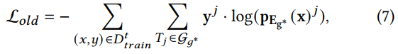
where y? and are vectors with lengths equal to the number of categories of the previous task ?? . The total loss is

 其中y? 和是向量的长度是否等于上一个任务的类别数?? . 全部损失是 

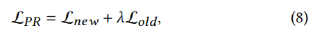
where ? is a hyper-parameter to balance training loss and distillation loss. Not that our method is without memory and does not require storing samples for previous tasks.

其中? 是平衡训练损失和蒸馏损失的超参数。并不是说我们的方法没有内存，也不需要存储以前任务的样本。 

Although the new task ?? is relevant to the task group G??, when the number of samples of the new task is far less than tasks in the group, it may cause the over-fitting of expert ???, leading to interference with previously accumulated knowledge in the expert. Therefore, we record the maximum number of samples of tasks in a task group. Suppose the maximum number in group G?? is ?, then, if the number of samples in the new task is less than 10 percent of ?, we fix the parameters of expert ??? and only the task-specific classification head is learnable. Since the new task is sufficiently relevant to the task group, by transferring the existing knowledge in expert ???, updating only the the classification header is sufficient to adapt to the new task.

虽然新任务?? 与工作组G??有关, 当新任务的样本数远远少于组中的任务时，可能会导致专家???的过度拟合, 导致干扰专家先前积累的知识。因此，我们记录任务组中任务的最大样本数。假设G??组中的最大数是?, 然后，如果新任务中的样本数小于?, 我们确定专家的参数??? 只有特定于任务的分类负责人是可学习的。由于新任务与任务组有足够的相关性，因此可以通过专家系统转移现有知识???, 仅更新分类头就足以适应新任务。

3.4 Parameter Allocation

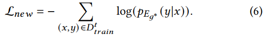
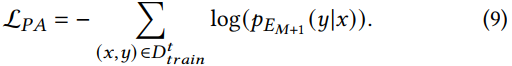
When all task groups are not relevant to the new task ?? , suppose the number of existing task groups is ?, we regard the new task as a new task group G?+1 and assign a new expert ??+1 for it. We adopt the cross-entropy for the classification problem and the loss function of task ?? is as follows:

当所有任务组与新任务不相关时?? , 假设现有任务组的数量为?, 我们将新任务视为一个新的任务组G?+1.指派新的专家??+1。我们采用交叉熵来处理分类问题，任务的损失函数?? 详情如下：

In our method, the number of experts and parameters are proportional to the number of task groups, mitigating the growth of parameter overhead. To further reduce the overhead of each expert, we adopt NAS to search for compact architectures for experts. Each expert in our method is stacked with multiple cells and the search for architecture is equivalent to the search for the appropriate cell. Since the time overhead of NAS becomes unbearable as the number of tasks increases, to improve the efficiency of architectural search in lifelong learning, we propose a relevance-aware sampling-based architecture search strategy. Specifically, as shown in Figure 2, we construct a hierarchical search space. The coarse-grained search space contains cells used by existing experts and an unknown cell which will be searched from the fine-grained search space. Following the common practice [26, 54], the fine-grained search space is a directed acyclic graph (DAG) with 7 nodes (two input nodes ?1,?2, an ordered sequence of intermediate nodes ?1, ?2, ?3, ?4, and an output node). The input nodes are defined as the outputs in the previous two layers and the output is concatenated from intermediate nodes. Each intermediate node is connected to all of its predecessors by directed candidate edges, which are associated with several candidate operations that are efficient in terms of the number of parameters.

在我们的方法中，专家和参数的数量与任务组的数量成正比，从而减少了参数开销的增长。为了进一步减少每个专家的开销，我们采用NAS为专家寻找紧凑的体系结构。我们方法中的每个专家都有多个单元，对架构的搜索相当于对适当单元的搜索。由于NAS的时间开销随着任务数量的增加而变得难以承受，为了提高终身学习中体系结构搜索的效率，我们提出了一种基于相关性感知采样的体系结构搜索策略。具体来说，如图2所示，我们构造了一个分层搜索空间。粗粒度搜索空间包含现有专家使用的单元格和将从细粒度搜索空间中搜索的未知单元格。按照惯例[26,54]，细粒度搜索空间是一个有7个节点（两个输入节点）的有向无环图（DAG）?1.?2.中间节点的有序序列?1.?2.?3.?4和一个输出节点）。输入节点定义为前两层中的输出，输出由中间节点连接而成。每个中间节点通过有向候选边连接到其所有前导节点，候选边与多个候选操作相关联，这些候选操作在参数数量上是有效的。 

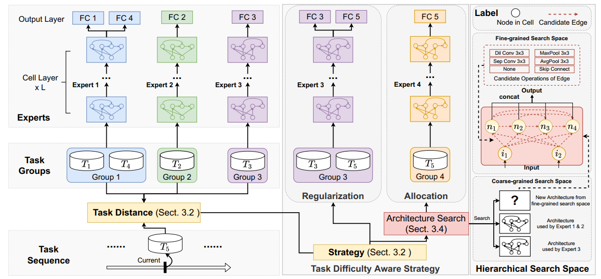
Figure 2: The architecture of Parameter Allocation & Regularization (PAR). Given a new task ?5, we first calculate the distance between it and existing task groups. Each task group has a expert shared by tasks in this group. Then we select a strategy from parameter regularization and parameter allocation according to the task distance. For parameter regularization, we add the new task into a task group and reuse the corresponding expert for it. For parameter allocation, we propose a architecture search strategy based on a hierarchical search space. The coarse-grained search space contains cells used by existing experts and an unknown cell which will be searched from the fine-grained search space. 

图2：参数分配和正则化（PAR）的体系结构。被赋予一项新任务?5。我们首先计算it与现有任务组之间的距离。每个任务组都有一名专家，由该组中的任务共享。然后根据任务距离从参数正则化和参数分配两个方面选择策略。对于参数正则化，我们将新任务添加到任务组中，并重用相应的专家。对于参数分配，我们提出了一种基于分层搜索空间的架构搜索策略。粗粒度搜索空间包含现有专家使用的单元格和将从细粒度搜索空间中搜索的未知单元格。

To search a cell for the new task, at first, we introduce a hyperparameter ?. When ≤ ?, we directly reuse the cell of expert ??? for the task ?? . A task distance greater than ? and less than ? indicates that the new task is not enough to share the expert with group G??, but can use the same architecture. When ??,?? > ?, we assign the unknown cell to the new expert and adopt an samplingbased NAS method MDL [54] to determine it. Specifically, for each candidate edge, we denote the probability, sampling epochs, and most recent performance of its candidate operations as ?, H?, and H? respectively, each of which is a real-valued column vector of length 8. We update them through multiple epochs of sampling to obtain a compact cell. In each epoch, to update H? and H?, we sample an operation for each edge to form a cell and evaluate it by training a model stacked by it one epoch. Then, to update the probability ?, we define the differential of sampling epochs as a 8×8 matrix ΔH? where. Similarly, we define the differential of performance as ΔH?. The probability ? is updated as follows:

为了在单元格中搜索新任务，我们首先引入一个超参数?。当 ≤ ?时, 为了完成任务?? ，我们直接重用专家的单元???。 任务距离大于? 不到? 表示新任务不足以与任务组G??共享专家, 但是可以使用相同的架构。当> ?时, 我们将未知单元格分配给新的专家，并采用基于抽样的NAS方法MDL[54]来确定它。具体来说，对于每个候选边，我们将其候选操作的概率、采样时间和最新性能分别表示为?, H?, H? ，每个都是长度为8的实值列向量。我们通过多次采样来更新它们，以获得一个紧凑的单元。在每个epoch，更新H? H?, 我们对每条边进行一次操作采样，形成一个单元，并通过训练一个由其叠加的模型来评估它。然后，更新概率?, 我们将采样周期的微分定义为8×8矩阵ΔH? 式中. 同样，我们将性能差定义为ΔH?. 概率? 更新如下：

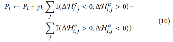
where ? is a hyper-parameter and I is the indicator function. The probabilities of operations with fewer sampling epochs and higher performance are enhanced and vice versa. For the final cell, operation with the highest probability in each edge is selected, then edges with top-2 probabilities for each intermediate node are used. The node value is equal to element-wise addition of results of these edges.

? 是一个超参数，I是指示函数。采样周期更少、性能更高的操作概率也会提高，反之亦然。对于最后一个小区，选择每个边缘中概率最高的操作，然后使用每个中间节点概率为 top-2 的边缘。节点值等于这些边的结果按元素相加。 

4 实验

4.1 Experimental Settings

Benchmarks. To evaluate the performance of our method, we conduct experiments on multiple benchmarks for task incremental learning. At first, we evaluate our method on two benchmarks containing a sequence of mixed similar and dissimilar tasks, including CTrL [47] and Mixed CIFAR100 and F-CelebA [19]. CTrL [47] includes 6 streams of visual image classification tasks. If ? is a task in the stream, CTrL denotes a task as ?? and ?+ whose data is sampled from the same distribution as ?, but with a much smaller or larger labeled dataset, respectively. Moreover, ? ′ and ? ′′ are tasks that are similar to task ?, while there are no relation between ?? and ?? for all ? ≠ ?. Then, the 6 streams in CTrl are as follows: ?? = (?1+, ?2, ?3, ?4, ?5, ?1?) is used to evaluate the ability of direct transfer; ?+ = (?1?, ?2, ?3, ?4, ?5, ?1+) is used to evaluate the ability of knowledge update; ?in = (?1, ?2, ?3, ?4, ?5, ?1′) and ?out = (?1, ?2, ?3, ?4, ?5, ?1′′) are used to evaluate the transfer to similar input and output distributions respectively; ?pl = (?1, ?2, ?3, ?4, ?5) is used to evaluate the plasticity; ?long consists of 100 tasks and is used to evaluate the scalability. Similarly, Mixed CIFAR100 and F-CelebA [19] including mixed similar tasks from F-CelebA and dissimilar tasks from CIFAR100 [21]. F-CelebA consists of 10 tasks selected from LEAF [5] that containing images of a celebrity labeled by whether he/she is smiling or not. CIFAR100 is split to 10 tasks and each task has 10 classes. Further, we conduct experiments on classical task incremental learning benchmarks including CIFAR10- 5, CIFAR100-10, CIFAR100-20 and MiniImageNet-20. CIFAR10-5 is constructed by dividing CIFAR10 [21] into 5 tasks and each task has 2 classes. Similarly, CIFAR100-10 and CIFAR100-20 are constructed by dividing CIFAR100 [21] into 10 tasks with 10 classes and 20 tasks with 5 classes respectively. MiniImageNet-20 is constructed by dividing MiniImageNet [48] into 20 tasks and each task has 5 classes.

基准。为了评估我们的方法的性能，我们在多个任务增量学习基准上进行了实验。首先，我们在包含一系列相似和不同任务的两个基准上评估我们的方法，包括CTrL[47]和mixed CIFAR100和F-CelebA[19]。CTrL[47]包括6个视觉图像分类任务流。如果? 是流中的任务，CTrL表示任务为?? 和?+ 其数据是从与?, 但分别使用更小或更大的标记数据集。此外? ′ 和? ′′ 是与任务类似的任务?, 虽然两者之间没有关系?? 和?? ,? ≠ ?。然后，CTrl中的6个流如下所示：?? = (?1+, ?2.?3.?4.?5.?1.?) 用于评估直接转移的能力；?+ = (?1.?, ?2.?3.?4.?5.?1+）用于评估知识更新能力；?in=(?1.?2.?3.?4.?5.?1′）和?out=(?1.?2.?3.?4.?5.?1′）分别用于评估向类似输入和输出分布的转移；?pl=(?1.?2.?3.?4.?5） 用于评估塑性；?long由100个任务组成，用于评估可伸缩性。类似地，混合的CIFAR100和F-CelebA[19]包括F-CelebA的混合相似任务和CIFAR100的不同任务[21]。F-CelebA由从LEAF[5]中选择的10个任务组成，其中包含一个名人的照片，该名人的标签是他/她是否在微笑。CIFAR100分为10个任务，每个任务有10个类。此外，我们还对经典的任务增量学习基准进行了实验，包括CIFAR10-5、CIFAR100-10、CIFAR100-20和MiniImageNet-20。CIFAR10-5将CIFAR10[21]划分为5个任务，每个任务有2个类。类似地，CIFAR100-10和CIFAR100-20是通过将CIFAR100[21]分为10个任务（10个类）和20个任务（5个类）来构建的。MiniImageNet-20将MiniImageNet[48]划分为20个任务，每个任务有5个类。

Baselines. We compare our method with: two simple baselines including Finetune that learns tasks one-by-one without any constraints and Independent that builds a model for each task independently; parameter regularization methods including EWC [20], LwF [25], IMM [23], and MAS [1]; memory based methods including iCaRL [37], ER [8], GCL [46], GPM [41], ACL [13], and OS (OrthogSubspace) [6]; parameter allocation method with static model: HAT[42], RPSnet [36], InstAParam [9], and CAT [19]; parameter allocation method with dynamic model: PN [40], Learn to Grow [24], SG-F [28], MNTDP [47], LMC [34], BNS [35], and FAS (Filter Atom Swapping) [30].

基线。我们将我们的方法与以下两个简单的基线进行比较：一个是Finetune，它在没有任何约束的情况下一个接一个地学习任务，另一个是独立的Finetune，它独立地为每个任务建立模型；参数正则化方法包括EWC[20]、LwF[25]、IMM[23]和MAS[1]；基于内存的方法包括iCaRL[37]、ER[8]、GCL[46]、GPM[41]、ACL[13]和OS（正交子空间）[6]；静态模型参数分配方法：HAT[42]、RPSnet[36]、InstAParam[9]和CAT[19]；具有动态模型的参数分配方法：PN[40]，Learn to Grow[24]，SG-F[28]，MNTDP[47]，LMC[34]，BNS[35]和FAS（滤波器原子交换）[30]。

Metrics. Denote the performance of the model on ?? as ??,? after learning task ?? where ? ≤ ?. Suppose the current task is ?? , we adopt average performance (AP) and average forgetting (AF) to evaluate lifelong learning methods. The formulas are as follows:

度量标准。当??,? 再学习任务??后表示在模型上的性能?? ，其中? ≤ ?. 假设当前任务是?? , 我们采用平均成绩（AP）和平均遗忘（AF）来评估终身学习方法。公式如下：

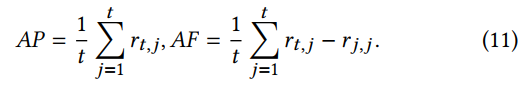
To evaluate the parameter overhead, we denote the initial and total number of model as M0 and M. The number of extra parameters for all new tasks is denoted as ΔM. The average number of extra parameters for each new task is denoted as ΔM.

为了评估参数开销，我们将模型的初始数量和总数表示为M0和M。所有新任务的额外参数数量表示为ΔM。每个新任务的额外参数平均数量表示为ΔM。

Implementation details. Our implementation is based on PyTorch and we provide the source code in the supplement. Without special instructions, we adopt a modified ResNet18 [17] with multiple output heads as the backbone network for baselines following MNTDP [47]. For our method, we set the number of cells of each expert as 4 for all tasks. The ? is set to 0.5 and ? is set to 1 for all tasks. We adopt the SGD optimizer and the initial learning rate is set to 0.01 and will be annealed following a cosine schedule. The momentum of SGD is set to 0.9 and the weight decay is searched from [0.0003, 0.001, 0.003, 0.01] according to the performance on valid data. Due to limited space, we provide detailed settings about dataset and experiments in the supplement.

实施细节。我们的实现是基于PyTorch的，我们在附录中提供了源代码。在没有特殊说明的情况下，我们采用了改进的ResNet18[17]，带有多个输出头，作为MNTDP[47]之后基线的主干网络。对于我们的方法，对于所有任务，我们将每个专家的单元数设置为4。这个? 设置为0.5和? 对于所有任务都设置为1。我们采用SGD优化器，初始学习率设置为0.01，并将按照余弦计划进行退火。SGD的动量设置为0.9，根据有效数据的性能，从[0.0003,0.001,0.003,0.01]搜索权重衰减。由于篇幅有限，我们在附录中提供了关于数据集和实验的详细设置。

4.2 Performance on Benchmarks

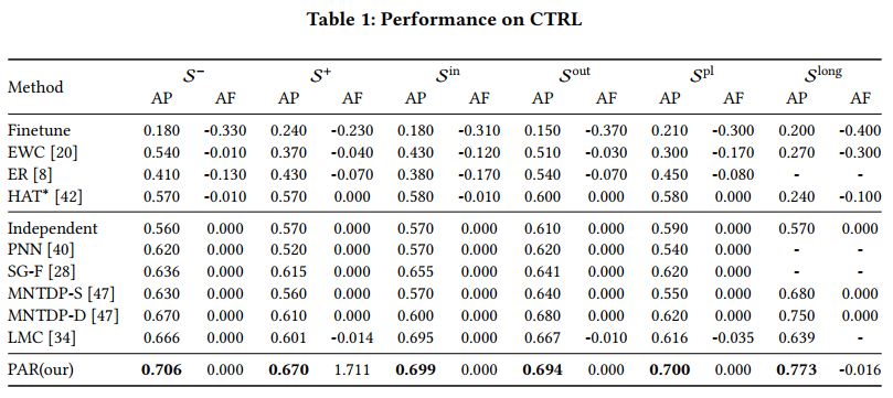
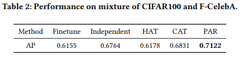
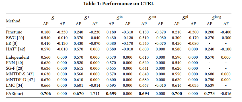
Performance mixed similar and dissimilar tasks. As shown in Table 1, parameter allocation methods via dynamic models perform better since they have enough new parameters to accommodate new tasks. Our method outperforms baselines on all six streams in CTrL. One reason is that our method allows knowledge transfer among relevant tasks while preventing interference among tasks not relevant. For example, performance on stream S+ show that our method can update the knowledge of expert for small task ?1? by the large task ?1+. Performance on streams S? and Sout shows that our method can transfer knowledge from experts of tasks that are relevant to last tasks. Another reason is that a task-tailored architecture helps each expert performs better. Moreover, performance on stream Slong shows that our method is scalable for the long task sequence. Similarly, results in Table 2 show that our method outperforms parameter allocation methods with static models.

性能混合了相似和不同的任务。如表1所示，通过动态模型的参数分配方法表现更好，因为它们有足够的新参数来适应新任务。我们的方法在CTrL中的所有六个流上都优于基线。一个原因是，我们的方法允许相关任务之间的知识转移，同时防止不相关任务之间的干扰。例如，在stream S+上的性能表明，我们的方法可以更新小任务的专家知识?1.? 大任务?1+. 流上的表现S?和 Sout表明，我们的方法可以从专家那里转移与最后一个任务相关的任务的知识。另一个原因是，任务定制的体系结构可以帮助每位专家更好地执行任务。此外，流Slong上的性能表明，我们的方法对于长任务序列是可伸缩的。类似地，表2中的结果表明，我们的方法优于静态模型的参数分配方法。

 

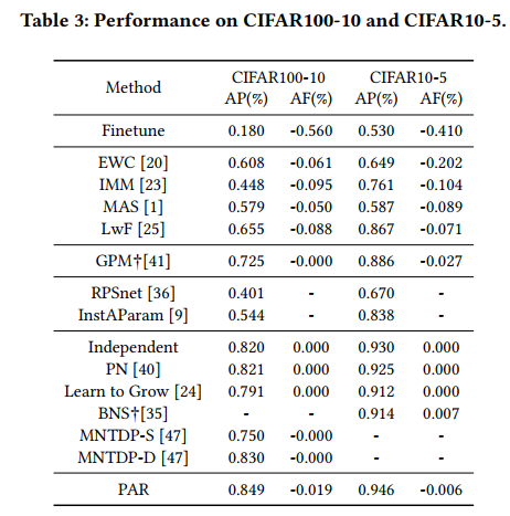
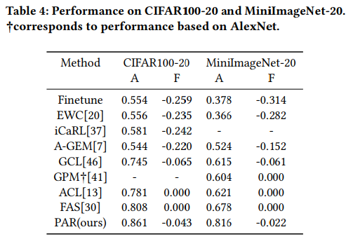
Performance on classical benchmarks. Experimental results in Table 3 and Table 4 show that our method outperforms baselines on 4 classical benchmarks. Thanks to the knowledge transfer and task-tailored architecture described above, despite slight forgetting, our method can achieve better performance on many tasks.

在经典基准上的表现。表3和表4中的实验结果表明，我们的方法在4个经典基准上优于基线。由于上述知识转移和任务定制架构，尽管有轻微的遗忘，我们的方法可以在许多任务上获得更好的性能。

 

Parameter overhead. We analyze the parameter overhead of our method on CIFAR100-10 and Slong in CTrL. The number of initial parameters (M0) in our method is large due to the extra feature extractor (ResNet18) for task distance calculation, but it is fixed and does not grow with the number of tasks. Compared with baselines, the total and average number of extra parameters for new tasks ΔM and ΔM in our method are small. Performance on stream Slong show that our method is scalable and the total parameter overhead in our method is less than baselines.

参数开销。我们在CIFAR100-10和CTrL上分析了我们的方法的参数开销。由于使用了额外的特征提取程序（ResNet18）来计算任务距离，我们的方法中的初始参数（M0）数量很大，但它是固定的，不随任务数量的增加而增加。与基线相比，我们的方法中新任务ΔM和ΔM的额外参数总数和平均数量都很小。流Slong上的性能表明，我们的方法是可伸缩的，并且我们的方法中的总参数开销小于基线。

4.3 Ablation Studies

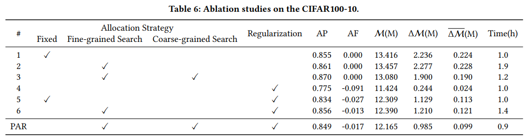
To analyze the effects of parameter allocation with relevance-aware architecture search and parameter regularization, we conduct ablation study on CIFAR100-10 and results are in Table 6. Compared with strategy Fixed, i.e. using a fixed cell from DARTs [26] in allocation, relevance-aware hierarchical search can improve the performance and reduce the parameter overhead. Moreover, the coarsegrained search based on relevance can further improve performance while reduce time overhead. We also find that the parameter regularization helps reduce parameter overhead, but it also degrades performance. Overall, our method achieves a balance among performance, parameter overhead, and time overhead.

为了分析相关感知架构搜索和参数正则化的参数分配效果，我们对CIFAR100-10进行了消融研究，结果如表6所示。与固定策略（即在分配中使用DART[26]中的固定单元）相比，相关感知分层搜索可以提高性能并减少参数开销。此外，基于相关性的粗粒度搜索可以进一步提高性能，同时减少时间开销。我们还发现，参数正则化有助于减少参数开销，但也会降低性能。总体而言，我们的方法在性能、参数开销和时间开销之间实现了平衡。

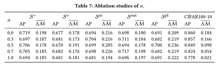
 We also analyze the effect of an important hyper-parameter ? on CTrL and CIFAR100-10. Results in Table 7 show that, on most tasks, the value of ? does not cause great performance changes, except the case that ? = 1.0 in CIFAR100-10.

我们还分析了一个重要的超参数的影响? 在CTrL和CIFAR100-10上。表7中的结果显示，在大多数任务中? 不会引起很大的性能变化，除非? = CIFAR100-10中的1.0。

 4.4 Relevance Analysis

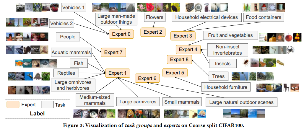
 Analysis on CIFAR100-coarse. In this section, we analyze the task relevance obtained by our method. At first, as shown in Figure 3, we visualize the tasks and experts in CIFAR100-coarse, which is obtained by dividing CIFAR100 into 20 tasks according to the coarsegrained labels in it. We find that Vechicles 1 and Vechicles 2, and Large man-made outdoor things share the same expert. The Aquatic mammals, Fish, Large carnivores, Large omnivores, herbivores, Medium-sized mammals, and Reptiles share the same expert. The People The containers and Household electrical devices share the same expert because they both contain cylindrical and circular objects. Non-insect invertebrates and Insects share the same expert because insects are invertebrates.

CIFAR100-coarse分析。在这一部分中，我们分析了通过我们的方法获得的任务相关性。首先，如图3所示，我们在CIFAR100粗略中可视化任务和专家，这是通过根据其中的粗粒度标签将CIFAR100划分为20个任务获得的。我们发现Vechicles 1和Vechicles 2，以及大型人造户外物品共享同一个专家。水生哺乳动物、鱼类、大型食肉动物、大型杂食动物、草食动物、中型哺乳动物和爬行动物都有相同的专家。容器和家用电器的使用者都是同一位专家，因为它们都包含圆柱形和圆形物体。非昆虫无脊椎动物和昆虫拥有相同的专家，因为昆虫是无脊椎动物。

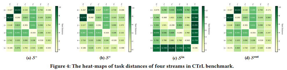
Analysis on CTrL. As shown in Figure 4, we visualize the heatmaps of task distances obtained by our method on 4 streams in ????. Results on streams S?, ?+ and Sout shot that our method can capture the similarities between tasks. 

对CTrL的分析。如图4所示，我们将通过我们的方法获得的任务距离热图可视化为????. 关于流的结果?, ?+ 我们的方法可以捕捉到任务之间的相似性。

5  结论

Instead of treating all tasks in a sequence equally and trying to solve them uniformly, in this paper, we propose a new lifelong learning framework named Parameter Allocation & Regularization (PAR) that allows the model to adaptively select an appropriate strategy from parameter allocation and parameter regularization for each task according to its learning difficulty. Experimental results on multiple benchmarks show that our method is scalable and significantly reduces the model redundancy while improving the model performance. Further, the relevance analyses show that the task relevance obtained by our method is reasonable and the model can automatically adopt the same expert to handle relevant tasks.

本文提出了一种新的终身学习框架，名为参数分配与正则化（PAR），该框架允许模型根据每个任务的学习难度，从参数分配和参数正则化中自适应地选择合适的策略，而不是将所有任务一视同仁，并试图统一地解决它们。在多个基准测试上的实验结果表明，该方法具有可扩展性，在提高模型性能的同时显著减少了模型冗余。此外，相关性分析表明，该方法得到的任务相关性是合理的，并且该模型可以自动采用同一专家来处理相关任务。