Homework 2 - Classification
�����κ����⣬��ӭ�������������� ntu-ml-2020spring-ta@googlegroups.com
Binary classification is one of the most fundamental problem in machine learning. In this tutorial, you are going to build linear binary classifiers to predict whether the income of an indivisual exceeds 50,000 or not. We presented a discriminative and a generative approaches, the logistic regression(LR) and the linear discriminant anaysis(LDA). You are encouraged to compare the differences between the two, or explore more methodologies. Although you can finish this tutorial by simpliy copying and pasting the codes, we strongly recommend you to understand the mathematical formulation first to get more insight into the two algorithms. Please find here and here for more detailed information about the two algorithms.
��Ԫ�����ǻ���ѧϰ�������������֮һ������ݽ�ѧ�У��㽫ѧ�����ʵ��һ�����Զ�Ԫ�����������������ǵĸ������ϣ��ж����������Ƿ���� 50,000 ��Ԫ�����ǽ������ַ���: logistic regression �� generative model�����������Ŀ�ģ�����Գ����˽⡢�������ߵ����������������������㷨�����ۻ��������Բο��������ʦ�Ľ�ѧͶӰƬ logistic regression �� generative model��
�����κ����⣬��ӭ�������������� ntu-ml-2020spring-ta@googlegroups.com
Dataset
This dataset is obtained by removing unnecessary attributes and balancing the ratio between positively and negatively labeled data in the Census-Income (KDD) Data Set, which can be found in UCI Machine Learning Repository. Only preprocessed and one-hot encoded data (i.e. X_train, Y_train and X_test) will be used in this tutorial. Raw data (i.e. train.csv and test.csv) are provided to you in case you are interested in it.
������ϼ����� UCI Machine Learning Repository �� Census-Income (KDD) Data Set ����һЩ������������Ϊ�˷���ѵ���������Ƴ���һЩ����Ҫ����Ѷ��������ƽ�����������ֱ�ǵı�������ʵ����ѵ�������У�ֻ�� X_train��Y_train �� X_test ���������������ĵ����ᱻʹ�õ���train.csv �� test.csv ������ԭʼ���ϵ�������ṩ��һЩ�������Ѷ��
Downloading...
From: https://drive.google.com/uc?id=1KSFIRh0-_Vr7SdiSCZP1ItV7bXPxMD92
To: /content/data.tar.gz
6.11MB [00:00, 53.2MB/s]
data/
data/sample_submission.csv
data/test_no_label.csv
data/train.csv
data/X_test
data/X_train
data/Y_train
data  data.tar.gz  sample_data
Logistic Regression
In this section we will introduce logistic regression first. We only present how to implement it here, while mathematical formulation and analysis will be omitted. You can find more theoretical detail in Prof. Lee's lecture.
�������ǻ�ʵ�� logistic regression���������ϸ��˵����ο��������ʦ�Ľ�ѧӰƬ
Preparing Data
Load and normalize data, and then split training data into training set and development set.
�������ϣ����Ҷ�ÿ�����������滯�����������ٽ����з�Ϊѵ�����뷢չ����
import numpy as npnp.random.seed(0)
X_train_fpath = './data/X_train'
Y_train_fpath = './data/Y_train'
X_test_fpath = './data/X_test'
output_fpath = './output_{}.csv'# Parse csv files to numpy array
with open(X_train_fpath) as f:next(f)X_train = np.array([line.strip('\n').split(',')[1:] for line in f], dtype = float)
with open(Y_train_fpath) as f:next(f)Y_train = np.array([line.strip('\n').split(',')[1] for line in f], dtype = float)
with open(X_test_fpath) as f:next(f)X_test = np.array([line.strip('\n').split(',')[1:] for line in f], dtype = float)def _normalize(X, train = True, specified_column = None, X_mean = None, X_std = None):# This function normalizes specific columns of X.# The mean and standard variance of training data will be reused when processing testing data.## Arguments:#     X: data to be processed#     train: 'True' when processing training data, 'False' for testing data#     specific_column: indexes of the columns that will be normalized. If 'None', all columns#         will be normalized.#     X_mean: mean value of training data, used when train = 'False'#     X_std: standard deviation of training data, used when train = 'False'# Outputs:#     X: normalized data#     X_mean: computed mean value of training data#     X_std: computed standard deviation of training dataif specified_column == None:specified_column = np.arange(X.shape[1])if train:X_mean = np.mean(X[:, specified_column] ,0).reshape(1, -1)X_std  = np.std(X[:, specified_column], 0).reshape(1, -1)X[:,specified_column] = (X[:, specified_column] - X_mean) / (X_std + 1e-8)return X, X_mean, X_stddef _train_dev_split(X, Y, dev_ratio = 0.25):# This function spilts data into training set and development set.train_size = int(len(X) * (1 - dev_ratio))return X[:train_size], Y[:train_size], X[train_size:], Y[train_size:]# Normalize training and testing data
X_train, X_mean, X_std = _normalize(X_train, train = True)
X_test, _, _= _normalize(X_test, train = False, specified_column = None, X_mean = X_mean, X_std = X_std)# Split data into training set and development set
dev_ratio = 0.1
X_train, Y_train, X_dev, Y_dev = _train_dev_split(X_train, Y_train, dev_ratio = dev_ratio)train_size = X_train.shape[0]
dev_size = X_dev.shape[0]
test_size = X_test.shape[0]
data_dim = X_train.shape[1]
print('Size of training set: {}'.format(train_size))
print('Size of development set: {}'.format(dev_size))
print('Size of testing set: {}'.format(test_size))
print('Dimension of data: {}'.format(data_dim))
Size of training set: 48830
Size of development set: 5426
Size of testing set: 27622
Dimension of data: 510Some Useful Functions
Some functions that will be repeatedly used when iteratively updating the parameters.
�⼸���������ܻ���ѵ�������б��ظ�ʹ�õ���
def _shuffle(X, Y):# This function shuffles two equal-length list/array, X and Y, together.randomize = np.arange(len(X))np.random.shuffle(randomize)return (X[randomize], Y[randomize])def _sigmoid(z):# Sigmoid function can be used to calculate probability.# To avoid overflow, minimum/maximum output value is set.return np.clip(1 / (1.0 + np.exp(-z)), 1e-8, 1 - (1e-8))def _f(X, w, b):# This is the logistic regression function, parameterized by w and b## Arguements:# X: input data, shape = [batch_size, data_dimension]# w: weight vector, shape = [data_dimension, ]# b: bias, scalar# Output:# predicted probability of each row of X being positively labeled, shape = [batch_size, ]return _sigmoid(np.matmul(X, w) + b)def _predict(X, w, b):# This function returns a truth value prediction for each row of X # by rounding the result of logistic regression function.return np.round(_f(X, w, b)).astype(np.int)def _accuracy(Y_pred, Y_label):# This function calculates prediction accuracyacc = 1 - np.mean(np.abs(Y_pred - Y_label))return accFunctions about gradient and loss
Please refers to Prof. Lee's lecture slides(p.12) for the formula of gradient and loss computation.
��ο��������ʦ�Ͽ�ͶӰƬ�� 12 ҳ���ݶȼ���ʧ�������㹫ʽ��
def _cross_entropy_loss(y_pred, Y_label):# This function computes the cross entropy.## Arguements:# y_pred: probabilistic predictions, float vector# Y_label: ground truth labels, bool vector# Output:# cross entropy, scalarcross_entropy = -np.dot(Y_label, np.log(y_pred)) - np.dot((1 - Y_label), np.log(1 - y_pred))return cross_entropydef _gradient(X, Y_label, w, b):# This function computes the gradient of cross entropy loss with respect to weight w and bias b.y_pred = _f(X, w, b)pred_error = Y_label - y_predw_grad = -np.sum(pred_error * X.T, 1)b_grad = -np.sum(pred_error)return w_grad, b_gradTraining
Everything is prepared, let's start training!
Mini-batch gradient descent is used here, in which training data are split into several mini-batches and each batch is fed into the model sequentially for losses and gradients computation. Weights and bias are updated on a mini-batch basis.
Once we have gone through the whole training set, the data have to be re-shuffled and mini-batch gradient desent has to be run on it again. We repeat such process until max number of iterations is reached.
����ʹ��С�����ݶ��½�����ѵ����ѵ�����ϱ���Ϊ����С���Σ����ÿһ��С���Σ����Ƿֱ�������ݶ��Լ���ʧ�������ݸ�����������ģ�͵IJ�������һ��ޒȦ��ɣ�Ҳ��������ѵ����������С���ζ���ʹ�ù�һ���Ժ����ǽ�����ѵ�����ϴ�ɢ�������·ֳ��µ�С���Σ�������һ��ޒȦ��ֱ�������趨��ޒȦ�������Ϊֹ��
# Zero initialization for weights ans bias
w = np.zeros((data_dim,))
b = np.zeros((1,))# Some parameters for training
max_iter = 10
batch_size = 8
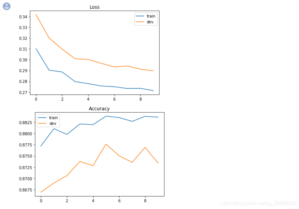
learning_rate = 0.2# Keep the loss and accuracy at every iteration for plotting
train_loss = []
dev_loss = []
train_acc = []
dev_acc = []# Calcuate the number of parameter updates
step = 1# Iterative training
for epoch in range(max_iter):# Random shuffle at the begging of each epochX_train, Y_train = _shuffle(X_train, Y_train)# Mini-batch trainingfor idx in range(int(np.floor(train_size / batch_size))):X = X_train[idx*batch_size:(idx+1)*batch_size]Y = Y_train[idx*batch_size:(idx+1)*batch_size]# Compute the gradientw_grad, b_grad = _gradient(X, Y, w, b)# gradient descent update# learning rate decay with timew = w - learning_rate/np.sqrt(step) * w_gradb = b - learning_rate/np.sqrt(step) * b_gradstep = step + 1# Compute loss and accuracy of training set and development sety_train_pred = _f(X_train, w, b)Y_train_pred = np.round(y_train_pred)train_acc.append(_accuracy(Y_train_pred, Y_train))train_loss.append(_cross_entropy_loss(y_train_pred, Y_train) / train_size)y_dev_pred = _f(X_dev, w, b)Y_dev_pred = np.round(y_dev_pred)dev_acc.append(_accuracy(Y_dev_pred, Y_dev))dev_loss.append(_cross_entropy_loss(y_dev_pred, Y_dev) / dev_size)print('Training loss: {}'.format(train_loss[-1]))
print('Development loss: {}'.format(dev_loss[-1]))
print('Training accuracy: {}'.format(train_acc[-1]))
print('Development accuracy: {}'.format(dev_acc[-1]))Training loss: 0.27135543524640593
Development loss: 0.2896359675026287
Training accuracy: 0.8836166291214418
Development accuracy: 0.8733873940287504
Plotting Loss and accuracy curve
import matplotlib.pyplot as plt# Loss curve
plt.plot(train_loss)
plt.plot(dev_loss)
plt.title('Loss')
plt.legend(['train', 'dev'])
plt.savefig('loss.png')
plt.show()# Accuracy curve
plt.plot(train_acc)
plt.plot(dev_acc)
plt.title('Accuracy')
plt.legend(['train', 'dev'])
plt.savefig('acc.png')
plt.show()
Predicting testing labels
Predictions are saved to output_logistic.csv.
Ԥ����Լ������ϱ�`���Ҵ��� output_logistic.csv �С�
# Predict testing labels
predictions = _predict(X_test, w, b)
with open(output_fpath.format('logistic'), 'w') as f:f.write('id,label\n')for i, label in  enumerate(predictions):f.write('{},{}\n'.format(i, label))# Print out the most significant weights
ind = np.argsort(np.abs(w))[::-1]
with open(X_test_fpath) as f:content = f.readline().strip('\n').split(',')
features = np.array(content)
for i in ind[0:10]:print(features[i], w[i])
Not in universe -4.031960278019251Spouse of householder -1.625403958705141Other Rel <18 never married RP of subfamily -1.4195759775765404Child 18+ ever marr Not in a subfamily -1.2958572076664745Unemployed full-time 1.1712558285885912Other Rel <18 ever marr RP of subfamily -1.167791807296237Italy -1.093458143800618Vietnam -1.0630365633146415
num persons worked for employer 0.9389922773566511 0.8226614922117185Porbabilistic generative model
In this section we will discuss a generative approach to binary classification. Again, we will not go through the formulation detailedly. Please find Prof. Lee's lecture if you are interested in it.
�������ǽ�ʵ������ generative model �Ķ�Ԫ������������ϸ����ο��������ʦ�Ľ�ѧӰƬ��
Preparing Data
Training and testing data is loaded and normalized as in logistic regression. However, since LDA is a deterministic algorithm, there is no need to build a development set.
ѵ��������Լ��Ĵ��������� logistic regression һģһ����Ȼ����Ϊ generative model �пɽ�������ѽ⣬��˲���ʹ�õ� development set��
# Parse csv files to numpy array
with open(X_train_fpath) as f:next(f)X_train = np.array([line.strip('\n').split(',')[1:] for line in f], dtype = float)
with open(Y_train_fpath) as f:next(f)Y_train = np.array([line.strip('\n').split(',')[1] for line in f], dtype = float)
with open(X_test_fpath) as f:next(f)X_test = np.array([line.strip('\n').split(',')[1:] for line in f], dtype = float)# Normalize training and testing data
X_train, X_mean, X_std = _normalize(X_train, train = True)
X_test, _, _= _normalize(X_test, train = False, specified_column = None, X_mean = X_mean, X_std = X_std)
Mean and Covariance
In generative model, in-class mean and covariance are needed.
�� generative model �У�������Ҫ�ֱ������������ڵ�����ƽ���빲���졣
# Compute in-class mean
X_train_0 = np.array([x for x, y in zip(X_train, Y_train) if y == 0])
X_train_1 = np.array([x for x, y in zip(X_train, Y_train) if y == 1])mean_0 = np.mean(X_train_0, axis = 0)
mean_1 = np.mean(X_train_1, axis = 0)  # Compute in-class covariance
cov_0 = np.zeros((data_dim, data_dim))
cov_1 = np.zeros((data_dim, data_dim))for x in X_train_0:cov_0 += np.dot(np.transpose([x - mean_0]), [x - mean_0]) / X_train_0.shape[0]
for x in X_train_1:cov_1 += np.dot(np.transpose([x - mean_1]), [x - mean_1]) / X_train_1.shape[0]# Shared covariance is taken as a weighted average of individual in-class covariance.
cov = (cov_0 * X_train_0.shape[0] + cov_1 * X_train_1.shape[0]) / (X_train_0.shape[0] + X_train_1.shape[0])
Computing weights and bias
Directly compute weights and bias from in-class mean and shared variance. Prof. Lee's lecture slides(p.33) gives a concise explanation.
Ȩ�ؾ�����ƫ����������ֱ�ӱ�����������㷨���Բο��������ʦ��ѧͶӰƬ�� 33 ҳ��
# Compute inverse of covariance matrix.
# Since covariance matrix may be nearly singular, np.linalg.inv() may give a large numerical error.
# Via SVD decomposition, one can get matrix inverse efficiently and accurately.
u, s, v = np.linalg.svd(cov, full_matrices=False)
inv = np.matmul(v.T * 1 / s, u.T)# Directly compute weights and bias
w = np.dot(inv, mean_0 - mean_1)
b =  (-0.5) * np.dot(mean_0, np.dot(inv, mean_0)) + 0.5 * np.dot(mean_1, np.dot(inv, mean_1))\+ np.log(float(X_train_0.shape[0]) / X_train_1.shape[0]) # Compute accuracy on training set
Y_train_pred = 1 - _predict(X_train, w, b)
print('Training accuracy: {}'.format(_accuracy(Y_train_pred, Y_train)))
Training accuracy: 0.8693232084930699Predicting testing labels
Predictions are saved to output_generative.csv.
Ԥ����Լ������ϱ�`���Ҵ��� output_generative.csv �С�
# Predict testing labels
predictions = 1 - _predict(X_test, w, b)
with open(output_fpath.format('generative'), 'w') as f:f.write('id,label\n')for i, label in  enumerate(predictions):f.write('{},{}\n'.format(i, label))# Print out the most significant weights
ind = np.argsort(np.abs(w))[::-1]
with open(X_test_fpath) as f:content = f.readline().strip('\n').split(',')
features = np.array(content)
for i in ind[0:10]:print(features[i], w[i])
29 -9.5791015625Forestry and fisheries 9.53662109375Retail trade 8.136718757 -7.81689453125Finance insurance and real estate 7.684570312541 -7.138671875Agriculture 6.97583007812534 -6.210937537 -5.6938476562533 -5.6201171875