版权声明:本文为CSDN博主「Nani_xiao」的原创文章,遵循 CC 4.0 BY-SA 版权协议,转载请附上原文出处链接及本声明。
原文链接:https://blog.csdn.net/xiao_lxl/article/details/90902323
很多深度学习网络训练都是在VGG-16, ZF-Net,Alex-Net,LeNet,Google-Net,ResNet, DenseNet-50框架的基础上进行训练的,现在把基于Keras框架下的这几个基础网络结构进行封装,方便需要时直接调用,或者在此基础上进行修改
以下导入前提可参考:
import numpy as np
#import tensorflow as tf
from keras import layers
from keras.layers import Input, Dense, Activation, ZeroPadding2D, BatchNormalization, Flatten, Conv2D
from keras.layers import AveragePooling2D, MaxPooling2D, Dropout, GlobalMaxPooling2D, GlobalAveragePooling2D
from keras.models import Model
from keras.preprocessing import image
from keras.utils import layer_utils
from keras.utils.data_utils import get_file
from keras.applications.imagenet_utils import preprocess_input
#import pydot
from IPython.display import SVG
from keras.utils.vis_utils import model_to_dot
from keras.utils import plot_model
from kt_utils import *
#import kt_utilsimport keras.backend as K
K.set_image_data_format('channels_last')
#import matplotlib.pyplot as plt
from matplotlib.pyplot import imshow
1.Keras封装实现 LeNet网络-5(1998)
LeNet-5模型诞生于1998年,是Yann LeCun教授在论文Gradient-based learning applied to document recognition中提出的,它是第一个成功应用于数字识别问题的卷积神经网络,麻雀虽小五脏俱全,它包含了深度学习的基本模块:卷积层,池化层,全连接层。是其他深度学习模型的基础。

LeNet除了输入层,总共有7层。输入是32*32大小的图像
C1是卷积层,卷积层的过滤器尺寸大小为55,深度为6,不使用全0补充,步长为1,所以这一层的输出尺寸为32-5+1=28,深度为6。
S2层是一个池化层,这一层的输入是C1层的输出,是一个28286的结点矩阵,过滤器大小为22,步长为2,所以本层的输出为14x14x6
C3层也是一个卷积层,本层的输入矩阵为14x14x6,过滤器大小为5x5,深度为16,不使用全0补充,步长为1,故输出为10x1016
S4层是一个池化层 ,输入矩阵大小为10x10x16,过滤器大小为2x2,步长为2,故输出矩阵大小为5x5*16
C5层是一个卷积层,过滤器大小为5x5,和全连接层没有区别,这里可看做全连接层。输入为5x5x16矩阵,将其拉直为一个长度为5x5x16的向量,即将一个三维矩阵拉直到一维向量空间中,输出结点为120。
F6层是全连接层 ,输入结点为120个,输出结点为84个
输出层也是全连接层,输入结点为84个,输出节点个数为10。
def LeNet():model = Sequential()model.add(Conv2D(32,(5,5),strides=(1,1),input_shape=(28,28,1),padding='valid',activation='relu',kernel_initializer='uniform'))model.add(MaxPooling2D(pool_size=(2,2)))model.add(Conv2D(64,(5,5),strides=(1,1),padding='valid',activation='relu',kernel_initializer='uniform'))model.add(MaxPooling2D(pool_size=(2,2)))model.add(Flatten())model.add(Dense(100,activation='relu'))model.add(Dense(10,activation='softmax'))return model
2.Keras封装实现 Alex-Net网络-8(2012)
2012年,AlexNet在ImageNet图像分类任务竞赛中获得冠军,一鸣惊人,从此开创了深度神经网络空前的高潮。论文ImageNet Classification with Deep Convolutional Neural Networks
AlexNet优势在于:
1.使用了非线性激活函数ReLU(如果不是很了解激活函数,可以参考我的另一篇博客 激活函数Activation Function,并验证其效果在较深的网络超过Sigmoid,成功解决了Sigmoid在网络较深时的梯度弥散问题。
2.提出了LRN(Local Response Normalization),局部响应归一化,LRN一般用在激活和池化函数后,对局部神经元的活动创建竞争机制,使其中响应比较大对值变得相对更大,并抑制其他反馈较小的神经元,增强了模型的泛化能力。
3.使用CUDA加速深度神经卷积网络的训练,利用GPU强大的并行计算能力,处理神经网络训练时大量的矩阵运算。
4.在CNN中使用重叠的最大池化,AlexNet全部使用最大池化,避免平均池化的模糊化效果。AlexNet中提出让步长比池化核的尺寸小,这样池化层的输出之间会有重叠和覆盖,提升了特征的丰富性。
5.使用数据增广(data agumentation)和Dropout防止过拟合。【数据增广】随机地从256256的原始图像中截取224224大小的区域,相当于增加了2048倍的数据量;【Dropout】AlexNet在后面的三个全连接层中使用Dropout,随机忽略一部分神经元,以避免模型过拟合。
Alex-Net包含了5个卷积层和2个全连接层。
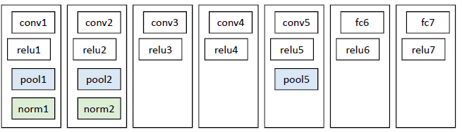
AlexNet总共包含8层,其中有5个卷积层和3个全连接层,有60M个参数,神经元个数为650k,分类数目为1000,LRN层出现在第一个和第二个卷积层后面,最大池化层出现在两个LRN层及最后一个卷积层后。
第一层输入图像规格为227x227x3,过滤器(卷积核)大小为11x11,深度为96,步长为4,则卷积后的输出为55x55x96,分成两组,进行池化运算处理,过滤器大小为3x3,步长为2,池化后的每组输出为27x27x48
第二层的输入为27x27x96,分成两组,为27x27x48,填充为2,过滤器大小为5x5,深度为128,步长为1,则每组卷积后的输出为27x27x128;然后进行池化运算,过滤器大小为3x3,步长为2,则池化后的每组输出为13x13x128
第三层两组中每组的输入为13x13x128,填充为1,过滤器尺寸为3x3,深度为192,步长为1,卷积后输出为13x13x192。在C3这里做了通道的合并,也就是一种串联操作,所以一个卷积核卷积的不再是单张显卡上的图像,而是两张显卡的图像串在一起之后的图像,所以卷积核的厚度为256,这也是为什么图上会画两个3x3x128的卷积核。
第四层两组中每组的输入为13x13x192,填充为1,过滤器尺寸为33,深度为192,步长为1,卷积后输出为13x13x192
第五层输入为上层的两组13x13x192,填充为1,过滤器大小为3x3,深度为128,步长为1,卷积后的输出为13x13x128;然后进行池化处理,过滤器大小为3x3,步长为2,则池化后的每组输出为6x6x128
第六层为全连接层,上一层总共的输出为6x6x256,所以这一层的输入为6x6x256,采用6x6x256尺寸的过滤器对输入数据进行卷积运算,每个过滤器对输入数据进行卷积运算生成一个结果,通过一个神经元输出,设置4096个过滤器,所以输出结果为4096
第六层的4096个数据与第七层的4096个神经元进行全连接
第八层的输入为4096,输出为1000(类别数目)
下面的代码运行在一块GPU上
def AlexNet():model = Sequential()model.add(Conv2D(96,(11,11),strides=(4,4),input_shape=(227,227,3),padding='valid',activation='relu',kernel_initializer='uniform'))model.add(MaxPooling2D(pool_size=(3,3),strides=(2,2)))model.add(Conv2D(256,(5,5),strides=(1,1),padding='same',activation='relu',kernel_initializer='uniform'))model.add(MaxPooling2D(pool_size=(3,3),strides=(2,2)))model.add(Conv2D(384,(3,3),strides=(1,1),padding='same',activation='relu',kernel_initializer='uniform'))model.add(Conv2D(384,(3,3),strides=(1,1),padding='same',activation='relu',kernel_initializer='uniform'))model.add(Conv2D(256,(3,3),strides=(1,1),padding='same',activation='relu',kernel_initializer='uniform'))model.add(MaxPooling2D(pool_size=(3,3),strides=(2,2)))model.add(Flatten())model.add(Dense(4096,activation='relu'))model.add(Dropout(0.5))model.add(Dense(4096,activation='relu'))model.add(Dropout(0.5))model.add(Dense(1000,activation='softmax'))return model
3.Keras封装实现 ZF-Net网络-8(2013)
ZF-Net网络包含了5个卷积层和2个全连接层
下图为AlexNet和ZF-Net的比较

F论文 Visualizing and Understanding Convolutional Networks 最大的贡献在于通过使用可视化技术揭示了神经网络各层到底在干什么,起到了什么作用。
可视化技术依赖于反卷积操作,即卷积的逆过程,将特征映射到像素上。具体过程如下图所示:
Unpooling:在卷积神经网络中,最大池化是不可逆的,作者采用近似的实现,使用一组转换变量switch 记录每个池化区域最大值的位置。在反池化的时候,将最大值返回到其所应该在的位置,其他位置用0补充。
Rectification:反卷积的时候也同样利用ReLU激活函数
Filtering:解卷积网络中利用卷积网络中相同的filter的转置应用到Rectified Unpooled Maps。也就是对filter进行水平方向和垂直方向的翻转。
可视化不仅能够看到一个训练完的模型的内部操作,而且还能够帮助改进网络结构从而提高网络性能。ZFNet模型是在AlexNet基础上进行改动,网络结构上并没有太大的突破。差异表现在, AlexNet是用两块GPU的稀疏连接结构,而ZFNet只用了一块GPU的稠密链接结构;改变了AleNet的第一层,将过滤器的大小由1111变成77,并且将步长由4变成2,使用更小的卷积核和步长,保留更多特征;将3,4,5层变成了全连接。

def ZF_Net():model = Sequential() model.add(Conv2D(96,(7,7),strides=(2,2),input_shape=(224,224,3),padding='valid',activation='relu',kernel_initializer='uniform')) model.add(MaxPooling2D(pool_size=(3,3),strides=(2,2))) model.add(Conv2D(256,(5,5),strides=(2,2),padding='same',activation='relu',kernel_initializer='uniform')) model.add(MaxPooling2D(pool_size=(3,3),strides=(2,2))) model.add(Conv2D(384,(3,3),strides=(1,1),padding='same',activation='relu',kernel_initializer='uniform')) model.add(Conv2D(384,(3,3),strides=(1,1),padding='same',activation='relu',kernel_initializer='uniform')) model.add(Conv2D(256,(3,3),strides=(1,1),padding='same',activation='relu',kernel_initializer='uniform')) model.add(MaxPooling2D(pool_size=(3,3),strides=(2,2))) model.add(Flatten()) model.add(Dense(4096,activation='relu')) model.add(Dropout(0.5)) model.add(Dense(4096,activation='relu')) model.add(Dropout(0.5)) model.add(Dense(1000,activation='softmax')) return model
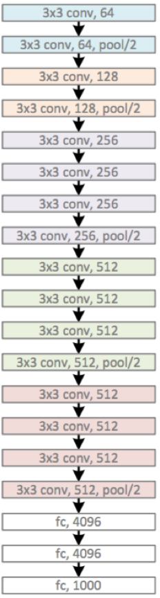
4.Keras封装实现 VGG-16网络 (2014)
4.1 VGG-16网络
Alex-Net包含了13个卷积层和3个全连接层。
conv层:2+2+3+3+3 = 13个
FC层:3个

VGG模型是牛津大学VGG组提出的。论文为Very Deep Convolutional Networks for Large-Scale Image Recognition VGG全部使用了3x3的卷积核和2x2最大池化核通过不断加深网络结构来提神性能。采用堆积的小卷积核优于采用大的卷积核,因为多层非线性层可以增加网络深层来保证学习更复杂的模式,而且所需的参数还比较少。
两个堆叠的卷积层(卷积核为3x3)有限感受野是5x5,三个堆叠的卷积层(卷积核为3x3)的感受野为7x7,故可以堆叠含有小尺寸卷积核的卷积层来代替具有大尺寸的卷积核的卷积层,并且能够使得感受野大小不变,而且多个3x3的卷积核比一个大尺寸卷积核有更多的非线性(每个堆叠的卷积层中都包含激活函数),使得decision function更加具有判别性。
假设一个3层的3x3卷积层的输入和输出都有C channels,堆叠的卷积层的参数个数为
而等同的一个单层的77卷积层的参数为

def VGG_16(): model = Sequential()model.add(Conv2D(64,(3,3),strides=(1,1),input_shape=(224,224,3),padding='same',activation='relu',kernel_initializer='uniform'))model.add(Conv2D(64,(3,3),strides=(1,1),padding='same',activation='relu',kernel_initializer='uniform'))model.add(MaxPooling2D(pool_size=(2,2)))model.add(Conv2D(128,(3,2),strides=(1,1),padding='same',activation='relu',kernel_initializer='uniform'))model.add(Conv2D(128,(3,3),strides=(1,1),padding='same',activation='relu',kernel_initializer='uniform'))model.add(MaxPooling2D(pool_size=(2,2)))model.add(Conv2D(256,(3,3),strides=(1,1),padding='same',activation='relu',kernel_initializer='uniform'))model.add(Conv2D(256,(3,3),strides=(1,1),padding='same',activation='relu',kernel_initializer='uniform'))model.add(Conv2D(256,(3,3),strides=(1,1),padding='same',activation='relu',kernel_initializer='uniform'))model.add(MaxPooling2D(pool_size=(2,2)))model.add(Conv2D(512,(3,3),strides=(1,1),padding='same',activation='relu',kernel_initializer='uniform'))model.add(Conv2D(512,(3,3),strides=(1,1),padding='same',activation='relu',kernel_initializer='uniform'))model.add(Conv2D(512,(3,3),strides=(1,1),padding='same',activation='relu',kernel_initializer='uniform'))model.add(MaxPooling2D(pool_size=(2,2)))model.add(Conv2D(512,(3,3),strides=(1,1),padding='same',activation='relu',kernel_initializer='uniform'))model.add(Conv2D(512,(3,3),strides=(1,1),padding='same',activation='relu',kernel_initializer='uniform'))model.add(Conv2D(512,(3,3),strides=(1,1),padding='same',activation='relu',kernel_initializer='uniform'))model.add(MaxPooling2D(pool_size=(2,2)))model.add(Flatten())model.add(Dense(4096,activation='relu'))model.add(Dropout(0.5))model.add(Dense(4096,activation='relu'))model.add(Dropout(0.5))model.add(Dense(1000,activation='softmax'))return model
4.2 VGG-19网络 (2014)
VGG-19网络结构 2014年
5.Keras封装实现 Google-Net网络-22(2014)
Inception
提高深度神经网络性能最直接的办法是增加它们尺寸,不仅仅包括深度(网络层数),还包括它的宽度,即每一层的单元个数。但是这种简单直接的解决方法存在两个重大的缺点,更大的网络意味着更多的参数,使得网络更加容易过拟合,而且还会导致计算资源的增大。经过多方面的思量,考虑到将稀疏矩阵聚类成相对稠密子空间来倾向于对稀疏矩阵的优化,因而提出inception结构。Google Inception Net是一个大家族,包括:
Inception v1结构(GoogLeNet):
论文为Going deeper with ConvolutionsGoogleNet为ILSVRC 2014比赛中的第一名,提出了Inception Module结构

Inception V2结构:
论文Batch Normalization: Accelerating Deep Network Training by Reducing Internal Covariate Shift Inception V2结构用两个33的卷积替代55的大卷机,提出了Batch Normalization(简称BN)正则化方法
Inception V2 其实在网络上没有什么改动,只是在输入的时候增加了batch_normal,所以他的论文名字也是叫batch_normal,加了这个以后训练起来收敛更快,学习起来自然更高效,可以减少dropout的使用。
其实也是个很简单的正则化处理,这样保证出现过的最大值为1,最小值为0,所有输出保证在0~1之间。
把55的卷积改成了两个33的卷积串联,它说一个55的卷积看起来像是一个55的全连接,所以干脆用两个3*3的卷积,第一层是卷积,第二层相当于全连接,这样可以增加网络的深度,并且减少了很多参数。

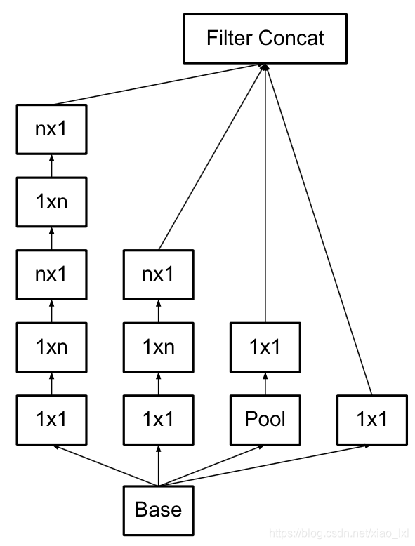
使用3×3的已经很小了,那么更小的2×2呢?2×2虽然能使得参数进一步降低,但是不如另一种方式更加有效,那就是Asymmetric方式,即使用1×3和3×1两种来代替3×3的卷积核。这种结构在前几层效果不太好,但对特征图大小为12~20的中间层效果明显。
Inception v3结构:
论文Rethinking the Inception Architecture for Computer Vision Inception V3 网络主要有两方面的改造:一是引入Factorization into small convolutions的思想,将较大的二维卷积拆分成两个较小的一维卷积,二是优化了Inception Module结构。
inception V3把googlenet里一些77的卷积变成了17和71的两层串联,33的也一样,变成了13和31,这样加速了计算,还增加了网络的非线性,减小过拟合的概率。另外,网络的输入从224改成了299.
Inception v4结构:
论文Inception-ResNet and the Impact of Residual Connections on learning Inception v4结构主要结合了微软的ResNet。
inception v4实际上是把原来的inception加上了resnet的方法,从一个节点能够跳过一些节点直接连入之后的一些节点,并且残差也跟着过去一个。
另外就是V4把一个先11再33那步换成了先33再11.
论文说引入resnet不是用来提高深度,进而提高准确度的,只是用来提高速度的。
Inception架构的主要思想是考虑怎样用容易获得密集组件近似覆盖卷积视觉网络的最优稀疏结构。Inception模型的基本结构如下,在多个不同尺寸的卷积核上同时进行卷积运算后再进行聚合,并使用1x1的卷积进行降维减少计算成本。 Inception Module使用了3中不同尺寸的卷积和1个最大池化,增加了网络对不同尺度的适应性。传统的卷集层的输入数据只和一种尺寸的卷积核进行运算,输出固定维度的特征数据(例如128),而在Inception模块中,输入和多个尺寸的卷积核(1x1,3x3和5x5)分别进行卷积运算,然后再聚合,输出的128特征中包括1x1卷积核的a1个输出特征,3x3卷积核的a2 个输出特征和5x5卷积核的a3个输出特征, (a1+a2+a3=128) 。Inception结构将相关性强的特征汇聚在一起,同样是128个输出特征,Inception得到的特征“冗余”的信息比较少,所以收敛速度就会更快。

GoogleNet
GoogleNet采用9个Inception模块化的结构,共22层,除了最后一层的输出,其中间结点的分类效果也很好。还使用了辅助类结点(auxiliary classifiers),将中间某一层的输出用作分类,并按一个较小的权重加到最终分类结果中。这样相当于做了模型融合,同时给网络增加了反向传播的梯度信号,也提供了额外的正则化,对于整个网络的训练大有益处。下图是网络的结构图:

注:每一个Inception结构模块包含两层

Inception V2结构 Inception V2参考VGG,用两个3x3的卷积代替5x5的大卷积,还提出著名的Batch Normalization(BN)方法。BN是一个非常有效的正则化方法,可以让大型卷积网络的训练速度加快很多倍,同时收敛后的分类准确率也可以得到大幅提高。BN用于神经网络某层时,会对每一个mini-batch数据进行标准化(normalization)处理,使输出规范化到N(0,1)的正态分布,减少了Internal Covariate shift(内部神经元的改变) 。
单纯地使用BN获得的增益还不明显,还需要对网络做一些相应的调整:增大学习率并加快学习衰减速度;去除Dropout和LRN并减轻L2 正则化;更彻底地对训练样本进行shuffle;减少数据增强中图片的光度失真,(BN网络训练很快,每一个样本训练样本训练次数更少,我们希望训练者关注更多真实的图片)

Inception v3结构 引入 Factorization into small convolutions的思想,将一个较大的二维卷积拆分成两个较小的一维卷积,比如将3x3卷积拆分成1x3和3x1卷积,一方面节约了大量参数,加速运算并减轻过拟合,同时增加了一层非线性扩展模型表达能力。这种非对称的卷积结构拆分,其结果比对称地拆为几个相同的小卷积核效果更明显,可以处理更多,更复杂的空间特征,增加特征多样性。另一方面,Inception V3优化了Inception Module结构,现在Inception Module有3535、1717和88三种不同的结构。
Inception v4结构 将Inception Module与Residual connection相结合,加速训练速度并提升性能。
def Conv2d_BN(x, nb_filter,kernel_size, padding='same',strides=(1,1),name=None):if name is not None:bn_name = name + '_bn'conv_name = name + '_conv'else:bn_name = Noneconv_name = Nonex = Conv2D(nb_filter,kernel_size,padding=padding,strides=strides,activation='relu',name=conv_name)(x)x = BatchNormalization(axis=3,name=bn_name)(x)return xdef Inception(x,nb_filter):branch1x1 = Conv2d_BN(x,nb_filter,(1,1), padding='same',strides=(1,1),name=None)branch3x3 = Conv2d_BN(x,nb_filter,(1,1), padding='same',strides=(1,1),name=None)branch3x3 = Conv2d_BN(branch3x3,nb_filter,(3,3), padding='same',strides=(1,1),name=None)branch5x5 = Conv2d_BN(x,nb_filter,(1,1), padding='same',strides=(1,1),name=None)branch5x5 = Conv2d_BN(branch5x5,nb_filter,(1,1), padding='same',strides=(1,1),name=None)branchpool = MaxPooling2D(pool_size=(3,3),strides=(1,1),padding='same')(x)branchpool = Conv2d_BN(branchpool,nb_filter,(1,1),padding='same',strides=(1,1),name=None)x = concatenate([branch1x1,branch3x3,branch5x5,branchpool],axis=3)return xdef GoogLeNet():inpt = Input(shape=(224,224,3))#padding = 'same',填充为(步长-1)/2,还可以用ZeroPadding2D((3,3))x = Conv2d_BN(inpt,64,(7,7),strides=(2,2),padding='same')x = MaxPooling2D(pool_size=(3,3),strides=(2,2),padding='same')(x)x = Conv2d_BN(x,192,(3,3),strides=(1,1),padding='same')x = MaxPooling2D(pool_size=(3,3),strides=(2,2),padding='same')(x)x = Inception(x,64)#256x = Inception(x,120)#480x = MaxPooling2D(pool_size=(3,3),strides=(2,2),padding='same')(x)x = Inception(x,128)#512x = Inception(x,128)x = Inception(x,128)x = Inception(x,132)#528x = Inception(x,208)#832x = MaxPooling2D(pool_size=(3,3),strides=(2,2),padding='same')(x)x = Inception(x,208)x = Inception(x,256)#1024x = AveragePooling2D(pool_size=(7,7),strides=(7,7),padding='same')(x)x = Dropout(0.4)(x)x = Dense(1000,activation='relu')(x)x = Dense(1000,activation='softmax')(x)model = Model(inpt,x,name='inception')return model
6.Keras封装实现 ResNet-50网络-34/50/101/152(2015)
论文Deep Residual Learning for Image Recognition
随着网络的加深,出现了训练集准确率下降,错误率上升的现象,就是所谓的“退化”问题。按理说更深的模型不应当比它浅的模型产生更高的错误率,这不是由于过拟合产生的,而是由于模型复杂时,SGD的优化变得更加困难,导致模型达不到好的学习效果。ResNet就是针对这个问题应运而生的。
ResNet,深度残差网络,基本思想是引入了能够跳过一层或多层的“shortcut connection”,如下图所示,即图中的“弯弯的弧线”。ResNet中提出了两种mapping:一种是identity mapping,另一种是residual mapping。最后的输出为y=F(x)+x,顾名思义,identity mapping指的是自身,也就是x,而residual mapping,残差,指的就是y-x=F(x)。这个简单的加法并不会给网络增加额外的参数和计算量,同时却能够大大增加模型的训练速度,提高训练效果,并且当模型的层数加深时,这个简单的结构能够很好的解决退化问题。

两种基础的残差设计:

这两种结构是分别针对ResNet34和ResNet50/101/152,右边的“bottleneck design”要比左边的“building block”多了1层,增添1*1的卷积目的就是为了降低参数的数目,减少计算量。所以浅层次的网络,可使用“building block”,对于深层次的网络,为了减少计算量,bottleneck desigh 是更好的选择。
再将x添加到F(x)中,还需考虑到x的维度与F(x)维度可能不匹配的情况,论文中给出三种方案:
A: 输入输出一致的情况下,使用恒等映射,不一致的情况下,则用0填充(zero-padding shortcuts)
B: 输入输出一致时使用恒等映射,不一致时使用 projection shortcuts
C: 在两种情况下均使用 projection shortcuts
经实验验证,虽然C要稍优于B,B稍优于A,但是A/B/C之间的稍许差异对解决“退化”问题并没有多大的贡献,而且使用0填充时,不添加额外的参数,可以保证模型的复杂度更低,这对更深的网络非常有利的,因此方法C被作者舍弃。
最后,放出一张图片展示常见的ResNet网络架构的组成,如下所示:

下面以50-layer的残差网络为例,展示ResNet的网络架构:
import Kerasdef Conv2d_BN(x, nb_filter,kernel_size, strides=(1,1), padding='same',name=None):if name is not None:bn_name = name + '_bn'conv_name = name + '_conv'else:bn_name = Noneconv_name = Nonex = Conv2D(nb_filter,kernel_size,padding=padding,strides=strides,activation='relu',name=conv_name)(x)x = BatchNormalization(axis=3,name=bn_name)(x)return xdef Conv_Block(inpt,nb_filter,kernel_size,strides=(1,1), with_conv_shortcut=False):x = Conv2d_BN(inpt,nb_filter=nb_filter[0],kernel_size=(1,1),strides=strides,padding='same')x = Conv2d_BN(x, nb_filter=nb_filter[1], kernel_size=(3,3), padding='same')x = Conv2d_BN(x, nb_filter=nb_filter[2], kernel_size=(1,1), padding='same')if with_conv_shortcut:shortcut = Conv2d_BN(inpt,nb_filter=nb_filter[2],strides=strides,kernel_size=kernel_size)x = add([x,shortcut])return xelse:x = add([x,inpt])return xdef ResNet50():inpt = Input(shape=(227,227,3))x = ZeroPadding2D((3,3))(inpt)x = Conv2d_BN(x,nb_filter=64,kernel_size=(7,7),strides=(2,2),padding='valid')x = MaxPooling2D(pool_size=(3,3),strides=(2,2),padding='same')(x)x = Conv_Block(x,nb_filter=[64,64,256],kernel_size=(3,3),strides=(1,1),with_conv_shortcut=True)x = Conv_Block(x,nb_filter=[64,64,256],kernel_size=(3,3))x = Conv_Block(x,nb_filter=[64,64,256],kernel_size=(3,3))x = Conv_Block(x,nb_filter=[128,128,512],kernel_size=(3,3),strides=(2,2),with_conv_shortcut=True)x = Conv_Block(x,nb_filter=[128,128,512],kernel_size=(3,3))x = Conv_Block(x,nb_filter=[128,128,512],kernel_size=(3,3))x = Conv_Block(x,nb_filter=[128,128,512],kernel_size=(3,3))x = Conv_Block(x,nb_filter=[256,256,1024],kernel_size=(3,3),strides=(2,2),with_conv_shortcut=True)x = Conv_Block(x,nb_filter=[256,256,1024],kernel_size=(3,3))x = Conv_Block(x,nb_filter=[256,256,1024],kernel_size=(3,3))x = Conv_Block(x,nb_filter=[256,256,1024],kernel_size=(3,3))x = Conv_Block(x,nb_filter=[256,256,1024],kernel_size=(3,3))x = Conv_Block(x,nb_filter=[256,256,1024],kernel_size=(3,3))x = Conv_Block(x,nb_filter=[512,512,2048],kernel_size=(3,3),strides=(2,2),with_conv_shortcut=True)x = Conv_Block(x,nb_filter=[512,512,2048],kernel_size=(3,3))x = Conv_Block(x,nb_filter=[512,512,2048],kernel_size=(3,3))x = AveragePooling2D(pool_size=(7,7))(x)x = Flatten()(x)x = Dense(1000,activation='softmax')(x)model = Model(inputs=inpt,outputs=x)return model
7.Keras封装实现 DenseNet-101网络(2016)


文章同时提出了DenseNet,DenseNet-B,DenseNet-BC三种结构,具体区别如下:
DenseNet:
Dense Block模块:BN+Relu+Conv(3*3)+dropout
transition layer模块:BN+Relu+Conv(11)(filternum:m)+dropout+Pooling(22)
DenseNet-B:
Dense Block模块:BN+Relu+Conv(11)(filternum:4K)+dropout+BN+Relu+Conv(33)+dropout
transition layer模块:BN+Relu+Conv(11)(filternum:m)+dropout+Pooling(22)
DenseNet-BC:
Dense Block模块:BN+Relu+Conv(11)(filternum:4K)+dropout+BN+Relu+Conv(33)+dropout
transition layer模块:BN+Relu+Conv(11)(filternum:θm,其中0<θ<1,文章取θ=0.5) +dropout +Pooling(22)
其中,DenseNet-B在原始DenseNet的基础上,加入Bottleneck layers, 主要是在Dense Block模块中加入了1*1卷积,使得将每一个layer输入的feature map都降为到4k的维度,大大的减少了计算量。
解决在Dense Block模块中每一层layer输入的feature maps随着层数增加而增大,则需要加入Bottleneck 模块,降维feature maps到4k维
DenseNet-BC在DenseNet-B的基础上,在transitionlayer模块中加入了压缩率θ参数,论文中将θ设置为0.5,这样通过1*1卷积,将上一个Dense Block模块的输出feature map维度减少一半。
import numpy as np
#import tensorflow as tf
from keras import layers
from keras.layers import Input, Dense, Activation, ZeroPadding2D, BatchNormalization, Flatten, Conv2D
from keras.layers import AveragePooling2D, MaxPooling2D, Dropout, GlobalMaxPooling2D, GlobalAveragePooling2D
from keras.models import Model
from keras.preprocessing import image
from keras.utils import layer_utils
from keras.utils.data_utils import get_file
from keras.applications.imagenet_utils import preprocess_input
#import pydot
from IPython.display import SVG
from keras.utils.vis_utils import model_to_dot
from keras.utils import plot_model
from kt_utils import *
#import kt_utilsimport keras.backend as K
K.set_image_data_format('channels_last')
#import matplotlib.pyplot as plt
from matplotlib.pyplot import imshow#%matplotlib inlinedef DenseNet121(nb_dense_block=4, growth_rate=32, nb_filter=64, reduction=0.0, dropout_rate=0.0, weight_decay=1e-4, classes=1000, weights_path=None):'''Instantiate the DenseNet 121 architecture,# Argumentsnb_dense_block: number of dense blocks to add to endgrowth_rate: number of filters to add per dense blocknb_filter: initial number of filtersreduction: reduction factor of transition blocks.dropout_rate: dropout rateweight_decay: weight decay factorclasses: optional number of classes to classify imagesweights_path: path to pre-trained weights# ReturnsA Keras model instance.'''eps = 1.1e-5# compute compression factorcompression = 1.0 - reduction# Handle Dimension Ordering for different backendsglobal concat_axisif K.image_dim_ordering() == 'tf':concat_axis = 3img_input = Input(shape=(224, 224, 3), name='data')else:concat_axis = 1img_input = Input(shape=(3, 224, 224), name='data')# From architecture for ImageNet (Table 1 in the paper)nb_filter = 64nb_layers = [6,12,24,16] # For DenseNet-121# Initial convolutionx = ZeroPadding2D((3, 3), name='conv1_zeropadding')(img_input)x = Convolution2D(nb_filter, 7, 7, subsample=(2, 2), name='conv1', bias=False)(x)x = BatchNormalization(epsilon=eps, axis=concat_axis, name='conv1_bn')(x)x = Scale(axis=concat_axis, name='conv1_scale')(x)x = Activation('relu', name='relu1')(x)x = ZeroPadding2D((1, 1), name='pool1_zeropadding')(x)x = MaxPooling2D((3, 3), strides=(2, 2), name='pool1')(x)# Add dense blocksfor block_idx in range(nb_dense_block - 1):stage = block_idx+2x, nb_filter = dense_block(x, stage, nb_layers[block_idx], nb_filter, growth_rate, dropout_rate=dropout_rate, weight_decay=weight_decay)# Add transition_blockx = transition_block(x, stage, nb_filter, compression=compression, dropout_rate=dropout_rate, weight_decay=weight_decay)nb_filter = int(nb_filter * compression)final_stage = stage + 1x, nb_filter = dense_block(x, final_stage, nb_layers[-1], nb_filter, growth_rate, dropout_rate=dropout_rate, weight_decay=weight_decay)x = BatchNormalization(epsilon=eps, axis=concat_axis, name='conv'+str(final_stage)+'_blk_bn')(x)x = Scale(axis=concat_axis, name='conv'+str(final_stage)+'_blk_scale')(x)x = Activation('relu', name='relu'+str(final_stage)+'_blk')(x)x = GlobalAveragePooling2D(name='pool'+str(final_stage))(x)x = Dense(classes, name='fc6')(x)x = Activation('softmax', name='prob')(x)model = Model(img_input, x, name='densenet')if weights_path is not None:model.load_weights(weights_path)return modeldef conv_block(x, stage, branch, nb_filter, dropout_rate=None, weight_decay=1e-4):'''Apply BatchNorm, Relu, bottleneck 1x1 Conv2D, 3x3 Conv2D, and option dropout# Argumentsx: input tensor stage: index for dense blockbranch: layer index within each dense blocknb_filter: number of filtersdropout_rate: dropout rateweight_decay: weight decay factor'''eps = 1.1e-5conv_name_base = 'conv' + str(stage) + '_' + str(branch)relu_name_base = 'relu' + str(stage) + '_' + str(branch)# 1x1 Convolution (Bottleneck layer)inter_channel = nb_filter * 4  x = BatchNormalization(epsilon=eps, axis=concat_axis, name=conv_name_base+'_x1_bn')(x)x = Scale(axis=concat_axis, name=conv_name_base+'_x1_scale')(x)x = Activation('relu', name=relu_name_base+'_x1')(x)x = Convolution2D(inter_channel, 1, 1, name=conv_name_base+'_x1', bias=False)(x)if dropout_rate:x = Dropout(dropout_rate)(x)# 3x3 Convolutionx = BatchNormalization(epsilon=eps, axis=concat_axis, name=conv_name_base+'_x2_bn')(x)x = Scale(axis=concat_axis, name=conv_name_base+'_x2_scale')(x)x = Activation('relu', name=relu_name_base+'_x2')(x)x = ZeroPadding2D((1, 1), name=conv_name_base+'_x2_zeropadding')(x)x = Convolution2D(nb_filter, 3, 3, name=conv_name_base+'_x2', bias=False)(x)if dropout_rate:x = Dropout(dropout_rate)(x)return xdef transition_block(x, stage, nb_filter, compression=1.0, dropout_rate=None, weight_decay=1E-4):''' Apply BatchNorm, 1x1 Convolution, averagePooling, optional compression, dropout # Argumentsx: input tensorstage: index for dense blocknb_filter: number of filterscompression: calculated as 1 - reduction. Reduces the number of feature maps in the transition block.dropout_rate: dropout rateweight_decay: weight decay factor'''eps = 1.1e-5conv_name_base = 'conv' + str(stage) + '_blk'relu_name_base = 'relu' + str(stage) + '_blk'pool_name_base = 'pool' + str(stage) x = BatchNormalization(epsilon=eps, axis=concat_axis, name=conv_name_base+'_bn')(x)x = Scale(axis=concat_axis, name=conv_name_base+'_scale')(x)x = Activation('relu', name=relu_name_base)(x)x = Convolution2D(int(nb_filter * compression), 1, 1, name=conv_name_base, bias=False)(x)if dropout_rate:x = Dropout(dropout_rate)(x)x = AveragePooling2D((2, 2), strides=(2, 2), name=pool_name_base)(x)return xdef dense_block(x, stage, nb_layers, nb_filter, growth_rate, dropout_rate=None, weight_decay=1e-4, grow_nb_filters=True):''' Build a dense_block where the output of each conv_block is fed to subsequent ones# Argumentsx: input tensorstage: index for dense blocknb_layers: the number of layers of conv_block to append to the model.nb_filter: number of filtersgrowth_rate: growth ratedropout_rate: dropout rateweight_decay: weight decay factorgrow_nb_filters: flag to decide to allow number of filters to grow'''eps = 1.1e-5concat_feat = xfor i in range(nb_layers):branch = i+1x = conv_block(concat_feat, stage, branch, growth_rate, dropout_rate, weight_decay)concat_feat = merge([concat_feat, x], mode='concat', concat_axis=concat_axis, name='concat_'+str(stage)+'_'+str(branch))if grow_nb_filters:nb_filter += growth_ratereturn concat_feat, nb_filter
总结
LeNet是第一个成功应用于手写字体识别的卷积神经网络 ALexNet展示了卷积神经网络的强大性能,开创了卷积神经网络空前的高潮
ZFNet通过可视化展示了卷积神经网络各层的功能和作用
VGG采用堆积的小卷积核替代采用大的卷积核,堆叠的小卷积核的卷积层等同于单个的大卷积核的卷积层,不仅能够增加决策函数的判别性还能减少参数量
GoogleNet增加了卷积神经网络的宽度,在多个不同尺寸的卷积核上进行卷积后再聚合,并使用1*1卷积降维减少参数量
ResNet解决了网络模型的退化问题,允许神经网络更深
注:关于AlexNet,GoogleNet,VGG和ResNet网络架构的demo代码见: