#
#作者:韦访
#博客:https://blog.csdn.net/rookie_wei
#微信:1007895847
#添加微信的备注一下是CSDN的
#欢迎大家一起学习
#
-----韦访 20190808
1、概述
标题不知道怎么取,就乱写了一个,这一讲,主要来玩玩英特尔的movidius神经计算棒(Intel Movidius Neural Compute Stick),就是下面这玩意,

插上电脑的USB接口,就可以用了,主要是用来跑神经网络的,传说中的VPU(Vision Processing Unit)。关于它的详细介绍自行百度,官方文档如下,
https://software.intel.com/en-us/movidius-ncs
https://movidius.github.io/ncsdk/index.html
我主要是玩它的ncsdk,用来加速神经网络的执行,需要注意的是,这玩意不能用来训练模型,所以没有GPU的想用它来代替GPU是不行的。这一讲,我们将tensorflow入门教程的第二讲的例子放到这上面来跑,第二讲链接如下,
https://blog.csdn.net/rookie_wei/article/details/80146620
2、安装
首先来安装ncsdk,官方安装教材链接如下,
https://movidius.github.io/ncsdk/install.html
很简单,如果是ubuntu系统,执行下面的命令行就可以了,
git clone -b ncsdk2 http://github.com/Movidius/ncsdk && cd ncsdk && sudo make install
其他系统或者环境的安装,自行看官方文档。
3、训练模型
安装完以后,就开始训练我们的CNN网络,来识别MNIST了,模仿官方教程来改我们自己的模型,官方教程链接如下,
https://movidius.github.io/ncsdk/tf_compile_guidance.html
我们的模型代码链接如下,
https://blog.csdn.net/rookie_wei/article/details/80146620
拖到底部,将完整代码拷贝到一个python文件mymnist.py里面,简单修改几个地方,将
x = tf.placeholder(tf.float32, [None, 784])
改为
x = tf.placeholder(tf.float32, [None, 784], name='input')
将
y_conv = tf.nn.softmax(tf.matmul(h_fc1_drop, W_fc2) + b_fc2)
改为
y_conv = tf.nn.softmax(tf.matmul(h_fc1_drop, W_fc2) + b_fc2, name='output')
也就是给输入输出占位符加了个名字,
完整代码如下,
# coding: utf-8
import tensorflow as tf
from tensorflow.examples.tutorials.mnist import input_data
import osos.environ['TF_CPP_MIN_LOG_LEVEL'] = '2'mnist = input_data.read_data_sets('mnist_data', one_hot=True)#初始化过滤器
def weight_variable(shape):return tf.Variable(tf.truncated_normal(shape, stddev=0.1))#初始化偏置,初始化时,所有值是0.1
def bias_variable(shape):return tf.Variable(tf.constant(0.1, shape=shape))#卷积运算,strides表示每一维度滑动的步长,一般strides[0]=strides[3]=1
#第四个参数可选"Same"或"VALID",“Same”表示边距使用全0填充
def conv2d(x, W):return tf.nn.conv2d(x, W, strides=[1, 1, 1, 1], padding="SAME")#池化运算
def max_pool_2x2(x):return tf.nn.max_pool(x, ksize=[1, 2, 2, 1], strides=[1, 2, 2, 1], padding="SAME")#创建x占位符,用于临时存放MNIST图片的数据,
# [None, 784]中的None表示不限长度,而784则是一张图片的大小(28×28=784)
x = tf.placeholder(tf.float32, [None, 784], name='input')
#y_存的是实际图像的标签,即对应于每张输入图片实际的值
y_ = tf.placeholder(tf.float32, [None, 10])#将图片从784维向量重新还原为28×28的矩阵图片,
# 原因参考卷积神经网络模型图,最后一个参数代表深度,
# 因为MNIST是黑白图片,所以深度为1,
# 第一个参数为-1,表示一维的长度不限定,这样就可以灵活设置每个batch的训练的个数了
x_image = tf.reshape(x, [-1, 28, 28, 1])#第一层卷积
#将过滤器设置成5×5×1的矩阵,
#其中5×5表示过滤器大小,1表示深度,因为MNIST是黑白图片只有一层。所以深度为1
#32表示我们要创建32个大小5×5×1的过滤器,经过卷积后算出32个特征图(每个过滤器得到一个特征图),即输出深度为64
W_conv1 = weight_variable([5, 5, 1, 32])
#有多少个特征图就有多少个偏置
b_conv1 = bias_variable([32])
#使用conv2d函数进行卷积计算,然后再用ReLU作为激活函数
h_conv1 = tf.nn.relu(conv2d(x_image, W_conv1) + b_conv1)
#卷积以后再经过池化操作
h_pool1 = max_pool_2x2(h_conv1)#第二层卷积
#因为经过第一层卷积运算后,输出的深度为32,所以过滤器深度和下一层输出深度也做出改变
W_conv2 = weight_variable([5, 5, 32, 64])
b_conv2 = bias_variable([64])
h_conv2 = tf.nn.relu(conv2d(h_pool1, W_conv2) + b_conv2)
h_pool2 = max_pool_2x2(h_conv2)#全连接层
#经过两层卷积后,图片的大小为7×7(第一层池化后输出为(28/2)×(28/2),
#第二层池化后输出为(14/2)×(14/2)),深度为64,
#我们在这里加入一个有1024个神经元的全连接层,所以权重W的尺寸为[7 * 7 * 64, 1024]
W_fc1 = weight_variable([7 * 7 * 64, 1024])
#偏置的个数和权重的个数一致
b_fc1 = bias_variable([1024])
#这里将第二层池化后的张量(长:7 宽:7 深度:64) 变成向量(跟上一节的Softmax模型的输入一样了)
h_pool2_flat = tf.reshape(h_pool2, [-1, 7 * 7 * 64])
#使用ReLU激活函数
h_fc1 = tf.nn.relu(tf.matmul(h_pool2_flat, W_fc1) + b_fc1)#dropout
#为了减少过拟合,我们在输出层之前加入dropout
keep_prob = tf.placeholder(tf.float32)
h_fc1_drop = tf.nn.dropout(h_fc1, keep_prob)#输出层
#全连接层输入的大小为1024,而我们要得到的结果的大小是10(0~9),
# 所以这里权重W的尺寸为[1024, 10]
W_fc2 = weight_variable([1024, 10])
b_fc2 = bias_variable([10])
#最后都要经过Softmax函数将输出转化为概率问题
y_conv = tf.nn.softmax(tf.matmul(h_fc1_drop, W_fc2) + b_fc2, name='output')#损失函数和损失优化
cross_entropy = tf.reduce_mean(-tf.reduce_sum(y_ * tf.log(y_conv)))
train_step = tf.train.AdamOptimizer(1e-4).minimize(cross_entropy)#测试准确率,跟Softmax回归模型的一样
correct_prediction = tf.equal(tf.argmax(y_conv, 1), tf.argmax(y_, 1))
accuracy = tf.reduce_mean(tf.cast(correct_prediction, tf.float32))#将训练结果保存,如果不保存我们这次训练结束后的结果也随着程序运行结束而释放了
savePath = './mnist_conv/'
saveFile = savePath + 'mnist_conv.ckpt'
if os.path.exists(savePath) == False:os.mkdir(savePath)saver = tf.train.Saver()#开始训练
with tf.Session() as sess:#初始化所有变量sess.run(tf.global_variables_initializer())#训练两万次for i in range(20000):#每次获取50张图片数据和对应的标签batch = mnist.train.next_batch(50)#每训练100次,我们打印一次训练的准确率if i % 100 == 0:train_accuracy =sess.run(accuracy, feed_dict={x:batch[0], y_:batch[1], keep_prob:1.0})print("step %d, training accuracy %g" % (i, train_accuracy))#这里是真的训练,将数据传入sess.run(train_step, feed_dict={x:batch[0], y_:batch[1], keep_prob:0.5})print ("end train, start testing...")mean_value = 0.0for i in range(mnist.test.labels.shape[0]):batch = mnist.test.next_batch(50)train_accuracy = sess.run(accuracy, feed_dict={x: batch[0], y_: batch[1], keep_prob: 1.0})mean_value += train_accuracyprint("test accuracy %g" % (mean_value / mnist.test.labels.shape[0]))# #训练结束后,我们使用mnist.test在测试最后的准确率# print("test accuracy %g" % sess.run(accuracy, feed_dict={x:mnist.test.images, y_:mnist.test.labels, keep_prob:1.0}))# 最后,将会话保存下来saver.save(sess, saveFile)
然后,就开始训练(前提是tensorflow环境要搭好),执行下面的命令行,
python3 mymnist.py
如果训练成功,会在当前文件夹下新增两个文件夹,
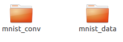
mnist_conv文件夹下有4个文件,就是我们训练的模型,这些都不了解的话,回去看教程。
4、重新保存模型
虽然上面我们已经训练出模型了,但是还不能直接使用,接下来,我们重新保存模型。将上面的代码保存到另一个python文件mymnist_inference.py里面,修改,
将
#y_存的是实际图像的标签,即对应于每张输入图片实际的值
y_ = tf.placeholder(tf.float32, [None, 10])
删除,
将
#dropout
#为了减少过拟合,我们在输出层之前加入dropout
keep_prob = tf.placeholder(tf.float32)
h_fc1_drop = tf.nn.dropout(h_fc1, keep_prob)
删除,
将
y_conv = tf.nn.softmax(tf.matmul(h_fc1_drop, W_fc2) + b_fc2, name='output')
改为,
y_conv = tf.nn.softmax(tf.matmul(h_fc1, W_fc2) + b_fc2, name='output')
将
#初始化所有变量
sess.run(tf.global_variables_initializer())
#训练两万次
for i in range(20000):
#每次获取50张图片数据和对应的标签
batch = mnist.train.next_batch(50)
#每训练100次,我们打印一次训练的准确率
if i % 100 == 0:
train_accuracy =sess.run(accuracy, feed_dict={x:batch[0], y_:batch[1], keep_prob:1.0})
print("step %d, training accuracy %g" % (i, train_accuracy))
#这里是真的训练,将数据传入
sess.run(train_step, feed_dict={x:batch[0], y_:batch[1], keep_prob:0.5})
print ("end train, start testing...")
mean_value = 0.0
for i in range(mnist.test.labels.shape[0]):
batch = mnist.test.next_batch(50)
train_accuracy = sess.run(accuracy, feed_dict={x: batch[0], y_: batch[1], keep_prob: 1.0})
mean_value += train_accuracy
print("test accuracy %g" % (mean_value / mnist.test.labels.shape[0]))
# #训练结束后,我们使用mnist.test在测试最后的准确率
# print("test accuracy %g" % sess.run(accuracy, feed_dict={x:mnist.test.images, y_:mnist.test.labels, keep_prob:1.0}))
# 最后,将会话保存下来
saver.save(sess, saveFile)
改为,
#初始化所有变量
sess.run(tf.global_variables_initializer())
sess.run(tf.local_variables_initializer())
saver.restore(sess, saveFile)
saver.save(sess, './model_inference' + '/mnist_inference')
完整代码如下,
# coding: utf-8
import tensorflow as tf
from tensorflow.examples.tutorials.mnist import input_data
import osos.environ['TF_CPP_MIN_LOG_LEVEL'] = '2'mnist = input_data.read_data_sets('mnist_data', one_hot=True)#初始化过滤器
def weight_variable(shape):return tf.Variable(tf.truncated_normal(shape, stddev=0.1))#初始化偏置,初始化时,所有值是0.1
def bias_variable(shape):return tf.Variable(tf.constant(0.1, shape=shape))#卷积运算,strides表示每一维度滑动的步长,一般strides[0]=strides[3]=1
#第四个参数可选"Same"或"VALID",“Same”表示边距使用全0填充
def conv2d(x, W):return tf.nn.conv2d(x, W, strides=[1, 1, 1, 1], padding="SAME")#池化运算
def max_pool_2x2(x):return tf.nn.max_pool(x, ksize=[1, 2, 2, 1], strides=[1, 2, 2, 1], padding="SAME")#创建x占位符,用于临时存放MNIST图片的数据,
# [None, 784]中的None表示不限长度,而784则是一张图片的大小(28×28=784)
x = tf.placeholder(tf.float32, [None, 784], name='input')#将图片从784维向量重新还原为28×28的矩阵图片,
# 原因参考卷积神经网络模型图,最后一个参数代表深度,
# 因为MNIST是黑白图片,所以深度为1,
# 第一个参数为-1,表示一维的长度不限定,这样就可以灵活设置每个batch的训练的个数了
x_image = tf.reshape(x, [-1, 28, 28, 1])#第一层卷积
#将过滤器设置成5×5×1的矩阵,
#其中5×5表示过滤器大小,1表示深度,因为MNIST是黑白图片只有一层。所以深度为1
#32表示我们要创建32个大小5×5×1的过滤器,经过卷积后算出32个特征图(每个过滤器得到一个特征图),即输出深度为64
W_conv1 = weight_variable([5, 5, 1, 32])
#有多少个特征图就有多少个偏置
b_conv1 = bias_variable([32])
#使用conv2d函数进行卷积计算,然后再用ReLU作为激活函数
h_conv1 = tf.nn.relu(conv2d(x_image, W_conv1) + b_conv1)
#卷积以后再经过池化操作
h_pool1 = max_pool_2x2(h_conv1)#第二层卷积
#因为经过第一层卷积运算后,输出的深度为32,所以过滤器深度和下一层输出深度也做出改变
W_conv2 = weight_variable([5, 5, 32, 64])
b_conv2 = bias_variable([64])
h_conv2 = tf.nn.relu(conv2d(h_pool1, W_conv2) + b_conv2)
h_pool2 = max_pool_2x2(h_conv2)#全连接层
#经过两层卷积后,图片的大小为7×7(第一层池化后输出为(28/2)×(28/2),
#第二层池化后输出为(14/2)×(14/2)),深度为64,
#我们在这里加入一个有1024个神经元的全连接层,所以权重W的尺寸为[7 * 7 * 64, 1024]
W_fc1 = weight_variable([7 * 7 * 64, 1024])
#偏置的个数和权重的个数一致
b_fc1 = bias_variable([1024])
#这里将第二层池化后的张量(长:7 宽:7 深度:64) 变成向量(跟上一节的Softmax模型的输入一样了)
h_pool2_flat = tf.reshape(h_pool2, [-1, 7 * 7 * 64])
#使用ReLU激活函数
h_fc1 = tf.nn.relu(tf.matmul(h_pool2_flat, W_fc1) + b_fc1)#输出层
#全连接层输入的大小为1024,而我们要得到的结果的大小是10(0~9),
# 所以这里权重W的尺寸为[1024, 10]
W_fc2 = weight_variable([1024, 10])
b_fc2 = bias_variable([10])
#最后都要经过Softmax函数将输出转化为概率问题
y_conv = tf.nn.softmax(tf.matmul(h_fc1, W_fc2) + b_fc2, name='output')#将训练结果保存,如果不保存我们这次训练结束后的结果也随着程序运行结束而释放了
savePath = './mnist_conv/'
saveFile = savePath + 'mnist_conv.ckpt'
if os.path.exists(savePath) == False:os.mkdir(savePath)saver = tf.train.Saver()#开始训练
with tf.Session() as sess:#初始化所有变量sess.run(tf.global_variables_initializer())  sess.run(tf.local_variables_initializer())      saver.restore(sess, saveFile)saver.save(sess, './model_inference' + '/mnist_inference')
在命令行中执行,
python3 mymnist_inference.py
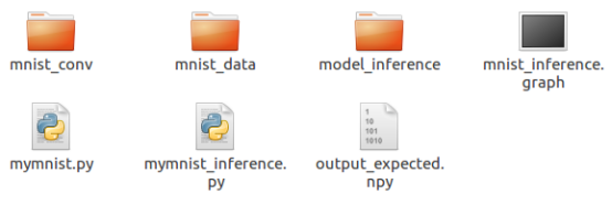
则当前文件夹下会新增一个名为model_inference的文件夹,文件夹下有4个文件,这个就是我们要的模型。上面的代码其实就是将模型部署时,不必要的占位符去掉,否则我们下一步要做的模型转换会出现问题。
5、模型转换
这一步,我们要将tensorflow模型转成ncsdk“认识”的模型,得到上面的模型以后,只要执行下面的命令即可,
mvNCCompile ./model_inference/mnist_inference.meta -s 12 -in input -on output -o mnist_inference.graph
执行完以后,如果顺利,在当前文件夹下会新增一个名为mnist_inference.graph的文件,这个就是我们要在神经计算棒上训练的模型。
6、在神经计算棒上运行模型
在当前文件夹下新建一个名为run_with_ncsdk2.py的python文件,加上如下代码,
from mvnc import mvncapi
import cv2
import numpy as np
# Get a list of available device identifiers
device_list = mvncapi.enumerate_devices()# Initialize a Device
device = mvncapi.Device(device_list[0])# Initialize the device and open communication
device.open()# Load graph file data
GRAPH_FILEPATH = './mnist_inference.graph'
with open(GRAPH_FILEPATH, mode='rb') as f:graph_buffer = f.read()# Initialize a Graph object
graph = mvncapi.Graph('mnist_graph')# Allocate the graph to the device and create input and output Fifos with default arguments
input_fifo, output_fifo = graph.allocate_with_fifos(device, graph_buffer)# Read an image from file
input_tensor = cv2.imread('4.jpg').astype(np.float32)
input_tensor = cv2.cvtColor(input_tensor, cv2.COLOR_RGB2GRAY)
print("input_tensor:", np.shape(input_tensor))
# Do pre-processing specific to this network model (resizing, subtracting network means, etc.)# Write the tensor to the input_fifo and queue an inference
graph.queue_inference_with_fifo_elem(input_fifo, output_fifo, input_tensor, 'output')# Get the results from the output queue
output, user_obj = output_fifo.read_elem()print("output:", output)
print("inference:", np.argmax(output))input_fifo.destroy()
output_fifo.destroy()
graph.destroy()
device.close()
device.destroy()
将我们要预测的4张mnist图片放到当前文件夹下,如下所示,
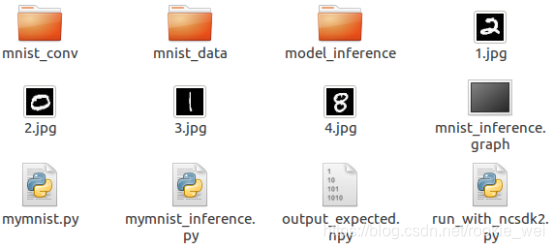
我们上面的代码要预测的是4.jpg图片里面的数字,执行如下命令,
python3 run_with_ncsdk2.py
运行结果如下,
input_tensor: (28, 28)
output: [ 0. 0. 0. 0. 0. 0. 0. 0. 1. 0.]
inference: 8
说明我们预测的结果是对的,我们的模型就这样在计算棒上运行了。怎么证明?你将计算棒拔了,再执行上面的命令看看。
上面所有源码下载链接:
https://download.csdn.net/download/rookie_wei/11501777