论文复现——Libra R-CNN: Towards Balanced Learning for Object Detection_综合

本次复现的论文已经开源了，不过是依赖mmdetection环境的。我有点小懒，当时没在学校的服务器上安装mmdetection，所以就自己复现了。
LibraRCNN官方开源代码：https://github.com/OceanPang/Libra_R-CNN
LibraRCNN原论文：https://arxiv.org/pdf/1904.02701.pdf
有些论文具体实现细节没有说清楚，所以我是按照自己的理解来复现的，如果有不同的方法欢迎在评论区讨论。

一、LibraRCNN结构

老样子，先上图：
在这里插入图片描述
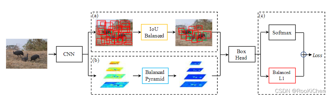
从上图可以看出来，LibraRCNN的整体框架跟FasterRCNN没什么区别，主要改进了三个部分：IoUBalanced、Balanced Pyramid、Banlanced L1，全文围绕Balanced，论文的名字Libra也是有天枰座的意思，下面就详细讲解一下这三个部分。

1.IoU Balanced

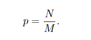
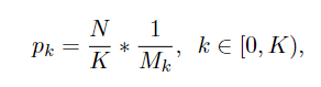
在原文中，作者说随机采样会忽视一部分负样本，导致样本不平衡，于是就将随机采样换成了分层采样，具体公式如下图：
随机采样
在这里插入图片描述
分层采样

原文中这里的K默认是3
在这里插入图片描述
这部分在代码实现时比较简单，但是会有一些细节需要处理：当框的数量不能被k整除时，需要将剩下的框全部采样。

这里贴一段IoU Balanced的实现代码，整个论文的具体代码可以参考文章末尾给出的链接。

# 分层采样# 首先将positive和negative分为三层
k = 3
# 每层有几个数据
pk = positive.numel() // 3
fk = negative.numel() // 3positive01 = positive[0:pk]
positive02 = positive[pk:pk * 2]
positive03 = positive[pk * 2:]negative01 = negative[0:fk]
negative02 = negative[fk:fk * 2]
negative03 = negative[fk * 2:]# 每层采集数据个数
num_pos_k = num_pos // 3
num_neg_k = num_neg // 3# 开始进行分层采样
rep01 = positive01[torch.randperm(positive01.numel(), device=positive.device)[:num_pos_k]]
rep02 = positive02[torch.randperm(positive02.numel(), device=positive.device)[:num_pos_k]]
rep03 = positive03[torch.randperm(positive03.numel(), device=positive.device)[:num_pos - 2*num_pos_k]]ref01 = negative01[torch.randperm(negative01.numel(), device=negative.device)[:num_neg_k]]
ref02 = negative02[torch.randperm(negative02.numel(), device=negative.device)[:num_neg_k]]
ref03 = negative03[torch.randperm(negative03.numel(), device=negative.device)[:num_neg - 2*num_neg_k]]pos_idx_per_image = torch.cat((rep01, rep02, rep03))
neg_idx_per_image = torch.cat((ref01, ref02, ref03))

2.Balanced Pyramid

在这里插入图片描述

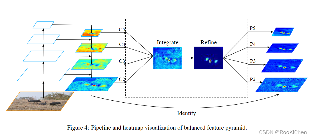
这里需要注意，作者将原来的Pi（i=2，3，4，5）写成了Ci（i=2，3，4，5），从图中也可以看出，Ci是经过上采样和特征融合得到的。特征图Integrate是由Ci经过线性插值和maxpool得到的，在Refine这个步骤中使用了Non-local，对于Non-local不了解的可以去阅读一下原论文：https://arxiv.org/abs/1711.07971v1，这里大致介绍一下Non-local：Non-local是self-attention在Non-local Net的应用，Non-local目的是获得全局的信息，可以理解为空间注意力机制（Non-local模块与Self-attention的之间的关系与区别）。为什么在这里使用Non-local呢，作者在原文中给出的解释是：由于特征图Integrate融合了多个尺度的信息，会导致严重的信息混淆，所以使用了非局部注意力的方法来进一步提高检测性能（原文说Refine这个步骤可以用3x3卷积层或Non-local，如果使用Non-local的话计算量有点大，但是使用3x3的卷积效果提升并不明显，所以最后我还是选择了使用Non-local）。在经过Refine后，还是使用线性插值和maxpool来得到Ri（i=2，3，4，5），并将Ci与Ri相加，得到最终的预测特征层。

3. Balanced L1

Balanced L1 loss 来自传统的smooth L1 loss，在该损失函数中，设置了一个拐点来分隔内值点和异常值，并将最大值为1.0的异常值产生的大梯度剪裁掉（如下图所示），这样做的目的是为了促进关键梯度的回归。
在这里插入图片描述
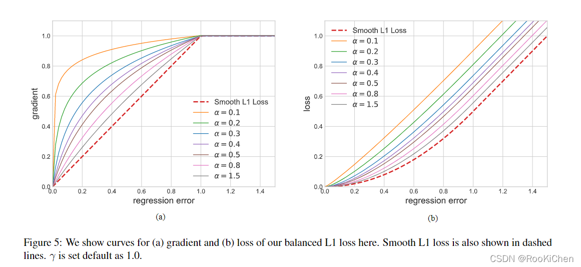
原文中给出了α和γ的具体值，只需要对下面的公式积分得到损失函数即可。

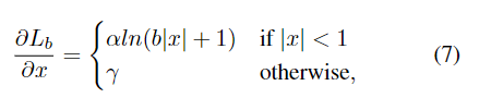
积分后可得损失函数L为：

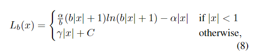
其中C是一个常数：C = γ / b - α * 1
这部分实现起来也比较简单，对着公式敲代码就完事了：

def balanced_l1_loss(input, target, beta=1.0, alpha=0.5, gamma=1.5):assert beta > 0assert input.size() == target.size() and target.numel() > 0diff = torch.abs(input - target)b = np.e ** (gamma / alpha) - 1loss = torch.where(diff < beta, alpha / b *(b * diff + 1) * torch.log(b * diff / beta + 1) - alpha * diff,gamma * diff + gamma / b - alpha * beta)return loss.sum()

我这里使用的是sum，是因为我在外面进行了mean，官方给出的代码是直接获得mean。

二、训练策略

用8个GPU(每个GPU 2个图像)对进行12轮的训练，初始学习率为0.02，如果没有具体说明，在第8和第11轮后分别将其下降0.1倍。其他超参数参考我的上一篇博客的代码：https://github.com/RooKichenn/CEFPN。没有8块卡的小伙伴可以用四块，每块4张图像，训练出来的效果没什么区别。

三、复现代码

代码已同步到GitHub，欢迎star：https://github.com/RooKichenn/LibraRCNN