Ŀ¼
- ǰ��
- 0��������Ҫ�İ��ͻ�������
- 1��Colors
- 2��plot_one_box��plot_one_box_PIL
-
- 2.1��plot_one_box
- 2.2��plot_one_box_PIL��û�õ���
- 3��plot_wh_methods��û�õ���
- 4��output_to_target��plot_images
-
- 4.1��output_to_target
- 4.1��plot_images
- 5��plot_lr_scheduler
- 6��hist2d��plot_test_txt��plot_targets_txt
-
- 6.1��hist2d
- 6.2��plot_test_txt
- 6.3��plot_targets_txt��û�õ���
- 7��plot_labels
- 8��plot_evolution
- 9��plot_results��plot_results_overlay��butter_lowpass_filtfilt
-
- 9.1��plot_results
- 9.2��plot_results_overlay
- 9.3��butter_lowpass_filtfilt
- 10��feature_visualization
- 11��plot_study_txt��û�õ�����profile_idetection��û�õ���
- �ܽ�
ǰ��
Դ�룺 YOLOv5Դ��.
����: ��YOLOV5-5.x Դ�뽲�⡿������Ŀ�ļ�����.
ע�Ͱ�ȫ����Ŀ�ļ����ϴ���GitHub: yolov5-5.x-annotations.
\qquad����ļ�����һЩ��ͼ��������һ�������ࡣ���뱾���������ѣ���Ҫ��һЩ���ĺ������ܴ��û�������������ܽ���һЩ��ͼ����һЩ�����Ļ�ͼ������ ��Opencv��ImageDraw��Matplotlib��Pandas��Seaborn��һЩ�����Ļ�ͼ��������������������������̫��Ļ�ͼ���������Բ�һ���ҵıʼǻ����Լ��ٶ�һ�¡�
0��������Ҫ�İ��ͻ�������
import glob # ��֧�ֲ���ͨ������ļ�����ģ��
import math # ��ѧ��ʽģ��
import os # �����ϵͳ���н�����ģ��
from copy import copy # �ṩͨ�õ�dz������copy����
from pathlib import Path # Path��strת��ΪPath���� ʹ�ַ���·�����ڲ�����ģ��import cv2 # opencv��
import matplotlib # matplotlibģ��
import matplotlib.pyplot as plt # matplotlib��ͼģ��
import numpy as np # numpy������������
import pandas as pd # pandas�������ģ��
import seaborn as sn # ����matplotlib��ͼ�ο��ӻ�python�� �ܹ�������������������ͳ��ͼ��
import torch # pytorch���
import yaml # yaml�����ļ���дģ��
from PIL import Image, ImageDraw, ImageFont # ͼƬ����ģ��
from torchvision import transforms # �����ܶ��ֶ�ͼ�����ݽ��б任�ĺ���from utils.general import increment_path, xywh2xyxy, xyxy2xywh
from utils.metrics import fitness# ����һЩ���������� Settings
matplotlib.rc('font', **{
'size': 11}) # �Զ���matplotlibͼ������font��Сsize=11
# ��PyCharm ҳ���п��ƻ�ͼ��ʾ���
# �����仰����import matplotlib.pyplot as plt֮ǰ�������plt.show()Ҳ��������Ļ�ϻ�ͼ ����֮����ʵûʲô��
matplotlib.use('Agg') # for writing to files only
1��Colors
\qquad����һ����ɫ�࣬����ѡ����Ӧ����ɫ�����续���ߵ���ɫ��������ɫ�ȵȡ�
Colors����룺
class Colors:# Ultralytics color palette https://ultralytics.com/def __init__(self):# hex = matplotlib.colors.TABLEAU_COLORS.values()hex = ('FF3838', 'FF9D97', 'FF701F', 'FFB21D', 'CFD231', '48F90A', '92CC17', '3DDB86', '1A9334', '00D4BB','2C99A8', '00C2FF', '344593', '6473FF', '0018EC', '8438FF', '520085', 'CB38FF', 'FF95C8', 'FF37C7')# ��hex�б�������hex��ʽ(ʮ������)����ɫת��rgb��ʽ����ɫself.palette = [self.hex2rgb('#' + c) for c in hex]# ��ɫ����self.n = len(self.palette)def __call__(self, i, bgr=False):# ���������index ѡ���Ӧ��rgb��ɫc = self.palette[int(i) % self.n]# ����ѡ�����ɫ Ĭ����rgbreturn (c[2], c[1], c[0]) if bgr else c@staticmethoddef hex2rgb(h): # rgb order (PIL)# hex -> rgbreturn tuple(int(h[1 + i:1 + i + 2], 16) for i in (0, 2, 4))colors = Colors() # ��ʼ��Colors���� �������colors��ʱ������__call__����
ʹ������Ҳ�DZȽϼ�ֻҪֱ��������ɫ��ż��ɣ�

2��plot_one_box��plot_one_box_PIL
\qquadplot_one_box �� plot_one_box_PIL ��������������������ԭͼim�ϻ�һ��bounding box����������ǰ��ʹ�õ���opencv������ʹ��PIL���������������Ĺ�����ʵ���ظ��ģ���ʵ�����õıȽ϶����plot_one_box������plot_one_box_PIL����û�ã��˽��¼��ɡ�
2.1��plot_one_box
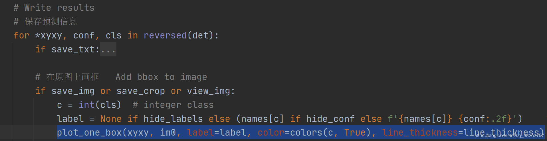
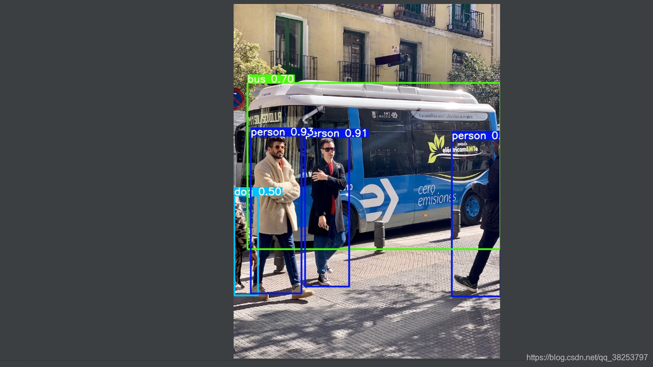
\qquad�������ͨ�����ڼ��nms��detect.py�У������յ�Ԥ��bounding box��ԭͼ�л����������������������ֻ�ܻ�һ�����
plot_one_box�������룺
def plot_one_box(x, im, color=(128, 128, 128), label=None, line_thickness=3):"""һ�������detect.py����nms֮�����ÿһ��Ԥ����ٽ�ÿ��Ԥ�����ԭͼ��ʹ��opencv��ԭͼim�ϻ�һ��bounding box:params x: Ԥ��õ���bounding box [x1 y1 x2 y2]:params im: ԭͼ Ҫ��bounding box�������ͼ�� array:params color: bounding box�ߵ���ɫ:params labels: ��ǩ�ϵĿ����Ϣ ��� + score:params line_thickness: bounding box���߿�"""# check im�ڴ��Ƿ�����assert im.data.contiguous, 'Image not contiguous. Apply np.ascontiguousarray(im) to plot_on_box() input image.'# tl = �����߿� Ҫô����line_thicknessҪô����ԭͼim������Ϣ����Ӧ����һ��tl = line_thickness or round(0.002 * (im.shape[0] + im.shape[1]) / 2) + 1 # line/font thickness# c1 = (x1, y1) = ���ο�����Ͻ� c2 = (x2, y2) = ���ο�����½�c1, c2 = (int(x[0]), int(x[1])), (int(x[2]), int(x[3]))# cv2.rectangle: ��im�ϻ������ c1: start_point(x1, y1) c2: end_point(x2, y2)# ע��: �����c1+c2���������Ͻ�+���½� Ҳ���������½�+���ϽǶ�����cv2.rectangle(im, c1, c2, color, thickness=tl, lineType=cv2.LINE_AA)# ���label��Ϊ�ջ�Ҫ�ڿ��������ʾ��ǩlabel + scoreif label:tf = max(tl - 1, 1) # label������߿� font thickness# cv2.getTextSize: ���������label��Ϣ�����ı��ַ����Ŀ��Ⱥ߶�# 0: ������������ fontScale: ��������ϵ�� thickness: ����ʻ��߿�# ����retval ����Ŀ��� (width, height), baseLine ���������ı��� y ����t_size = cv2.getTextSize(label, 0, fontScale=tl / 3, thickness=tf)[0]c2 = c1[0] + t_size[0], c1[1] - t_size[1] - 3# ͬ����һ���Ǹ�����IJ��� �����߿�thickness=-1��ʾ�������ζ����color��ɫcv2.rectangle(im, c1, c2, color, -1, cv2.LINE_AA) # filled# cv2.putText: ��ͼƬ��д�ı� ������������������ο���дlabel + score�ı�# (c1[0], c1[1] - 2)�ı����½����� 0: ������ʽ fontScale: ��������ϵ��# [225, 255, 255]: ������ɫ thickness: tf����ʻ��߿� lineType: ����ʽcv2.putText(im, label, (c1[0], c1[1] - 2), 0, tl / 3, [225, 255, 255], thickness=tf, lineType=cv2.LINE_AA)
�������һ�������detect.py����nms֮�����ÿһ��Ԥ����ٽ�ÿ��Ԥ�����ԭͼ���磺
Ч��������ʾ��
2.2��plot_one_box_PIL��û�õ���
\qquad�����������PIL��ԭͼ�л�һ�������ú�plot_one_boxһ������������һ�㶼����plot_one_box��������������������˽��¼��ɡ�
plot_one_box_PIL�������룺
def plot_one_box_PIL(box, im, color=(128, 128, 128), label=None, line_thickness=None):"""ʹ��PIL��ԭͼim�ϻ�һ��bounding box:params box: Ԥ��õ���bounding box [x1 y1 x2 y2]:params im: ԭͼ Ҫ��bounding box�������ͼ�� array:params color: bounding box�ߵ���ɫ:params label: ��ǩ�ϵ�bounding box�����Ϣ ��� + score:params line_thickness: bounding box���߿�"""# ��ԭͼarray��ʽ->Image��ʽim = Image.fromarray(im)# (��ʼ��)����һ�������ڸ���ͼ��(im)�ϻ�ͼ�Ķ���, ��֮�����draw.������ʱ����Ҫ����im����������ֱ�����im�Ͻ��л滭��draw = ImageDraw.Draw(im)# ���û���bounding box���߿�line_thickness = line_thickness or max(int(min(im.size) / 200), 2)# ��imͼ���ϻ���bounding box# xy: box [x1 y1 x2 y2] ���Ͻ� + ���½� width: �߿� outline: ���������ɫcolor fill: ���������������ɫcolor# outline��fillһ����������ѡһdraw.rectangle(box, width=line_thickness, outline=color) # plot# ���label��Ϊ�ջ�Ҫ�ڿ��������ʾ��ǩlabel + scoreif label:# ����һ��TrueType����OpenType�����ļ�("Arial.ttf"), ���Ҵ���һ���������font, fontд���������Сsize=12font = ImageFont.truetype("Arial.ttf", size=max(round(max(im.size) / 40), 12))# ���ظ����ı�label�Ŀ���txt_width�߶�txt_heighttxt_width, txt_height = font.getsize(label)# ��imͼ���ϻ��ƾ��ο� ������������ɫcolor(�������label��Ϣ) [x1 y1 x2 y2] ���Ͻ� + ���½�draw.rectangle([box[0], box[1] - txt_height + 4, box[0] + txt_width, box[1]], fill=color)# ���������������д��text��Ϣ(label) x1y1 ���Ͻ�draw.text((box[0], box[1] - txt_height + 1), label, fill=(255, 255, 255), font=font)# �ٷ���array���͵�im(���bounding box��label��)return np.asarray(im)
3��plot_wh_methods��û�õ���
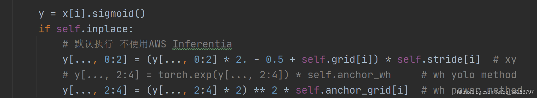
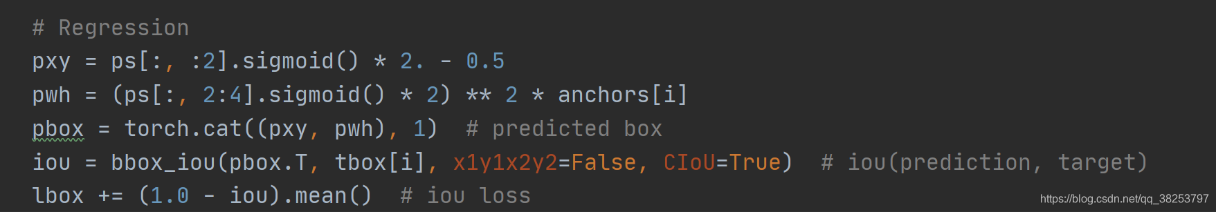
\qquad���������Ҫ�������Ƚ� ya=exy_a = e^xya?=ex �� yb=(2?sigmoid(x))2y_b = (2 * sigmoid(x))^2yb?=(2?sigmoid(x))2 �� yc=(2?sigmoid(x))1.6y_c = (2 * sigmoid(x))^{1.6}yc?=(2?sigmoid(x))1.6 ����������ͼ�εġ����� yay_aya? ����ͨ��yolo method��yby_byb? �� ycy_cyc?�����������powe method�������� https://github.com/ultralytics/yolov3/issues/168.�У����������۹����issue��������ʵ���з���ʹ��ԭ����yolo method��ʧ������ʱ���ͻȻѸ����������Noneֵ, ��power method��ʽ����wh��ʧ�½���Ƚ�ƽ�ȡ����ʵ��֤�� yby_byb? ����õ�wh��ʧ���㷽ʽ, yolov5��wh��ʧ��������õľ��� yby_byb? ���㷽ʽ �磺
yolo.py��
loss.py��
plot_wh_methods�������룺
def plot_wh_methods():"""û�õ��Ƚ�ya=e^x��yb=(2 * sigmoid(x))^2 �Լ� yc=(2 * sigmoid(x))^1.6 ����ͼ��wh��ʧ����ķ�ʽya��yb��yc���� ya: yolo method yb/yc: power methodʵ�鷢��ʹ��ԭ����yolo method��ʧ������ʱ���ͻȻѸ����������Noneֵ, ��power method��ʽ����wh��ʧ�½���Ƚ�ƽ�����ʵ��֤��yb����õ�wh��ʧ���㷽ʽ, yolov5��wh��ʧ��������õľ���yb���㷽ʽCompares the two methods for width-height anchor multiplicationhttps://github.com/ultralytics/yolov3/issues/168"""x = np.arange(-4.0, 4.0, .1) # (-4.0, 4.0) ÿ��0.1ȡһ��ֵya = np.exp(x) # ya = e^x yolo methodyb = torch.sigmoid(torch.from_numpy(x)).numpy() * 2 # yb = 2 * sigmoid(x)fig = plt.figure(figsize=(6, 3), tight_layout=True) # �����Զ���ͼ�� ��ʼ������plt.plot(x, ya, '.-', label='YOLOv3') # ��������ͼ ��������Ӽ�����plt.plot(x, yb ** 2, '.-', label='YOLOv5 ^2')plt.plot(x, yb ** 1.6, '.-', label='YOLOv5 ^1.6')plt.xlim(left=-4, right=4) # ����x�ᡢy�᷶Χplt.ylim(bottom=0, top=6)plt.xlabel('input') # ����x�ᡢy���ǩplt.ylabel('output')plt.grid() # ��������plt.legend() # ����ͼ�� ���������ͼ����Ҫ��plt.plot�м���label����(ͼ����)fig.savefig('comparison.png', dpi=200) # plt����ͼ, fig.savefig()����ͼƬ
\qquad��ʵ��������������ر���Ҫ��ֻ�ǿ��ӻ�һ���������������������ǵ������ڴ�����Ҳû���ù���������������˽��������� wh ��ʧ����ķ�ʽ��Power Method�����Ǻ��б�Ҫ�ġ�
4��output_to_target��plot_images
\qquad������������ʵҲ�ǶԼ���Ŀ���ʽ���д�����output_to_target��Ȼ���ٽ��仭����ʾ��ԭͼ�ϣ�plot_images������������������������test.py�еģ���Ե�Ҳ������һ��ͼƬһ����������batch�е����п���plot_images�Ὣ����batch��ͼƬ������һ�Ŵ�ͼmosaic�У������µľ�ɾ������Щ����plot_images������plot_one_box������
4.1��output_to_target
\qquad������������ڽ�����nms���output [num_obj��x1y1x2y2+conf+cls] -> [num_obj��batch_id+class+xywh+conf]�������漰��ͼ����������ת��predict�ĸ�ʽ��ͨ�����ڻ�ͼ����plot_images֮ǰ��
output_to_target�������룺
def output_to_target(output):"""����test.py�н��л���ǰ3��batch��Ԥ���predictions ��Ϊֻ��predictions��Ҫ�ĸ�ʽ target�Dz���Ҫ�ĸ�ʽ�Ľ�����nms���output [num_obj��x1y1x2y2+conf+cls] -> [num_obj, batch_id+class+x+y+w+h+conf] ת���ʽ�Ա���plot_images�н��л�ͼ + ��ʾlabelConvert model output to target format [batch_id, class_id, x, y, w, h, conf]:params output: list{tensor(8)}�ֱ��Ӧ�ŵ�ǰbatch��8(batch_size)��ͼƬ����nms��Ľ��list��ÿ��tensor[n, 6] n��ʾ��ǰͼƬ����Ŀ����� 6=x1y1x2y2+conf+cls:return np.array(targets): [num_targets, batch_id+class+xywh+conf] ����num_targetsΪ��ǰbatch�����м�Ŀ���ĸ���"""targets = []for i, o in enumerate(output): # ��ÿ��ͼƬ�ֱ�������for *box, conf, cls in o.cpu().numpy(): # ��ÿ��ͼƬ��ÿ������Ŀ������convert��ʽtargets.append([i, cls, *list(*xyxy2xywh(np.array(box)[None])), conf])return np.array(targets)
4.1��plot_images
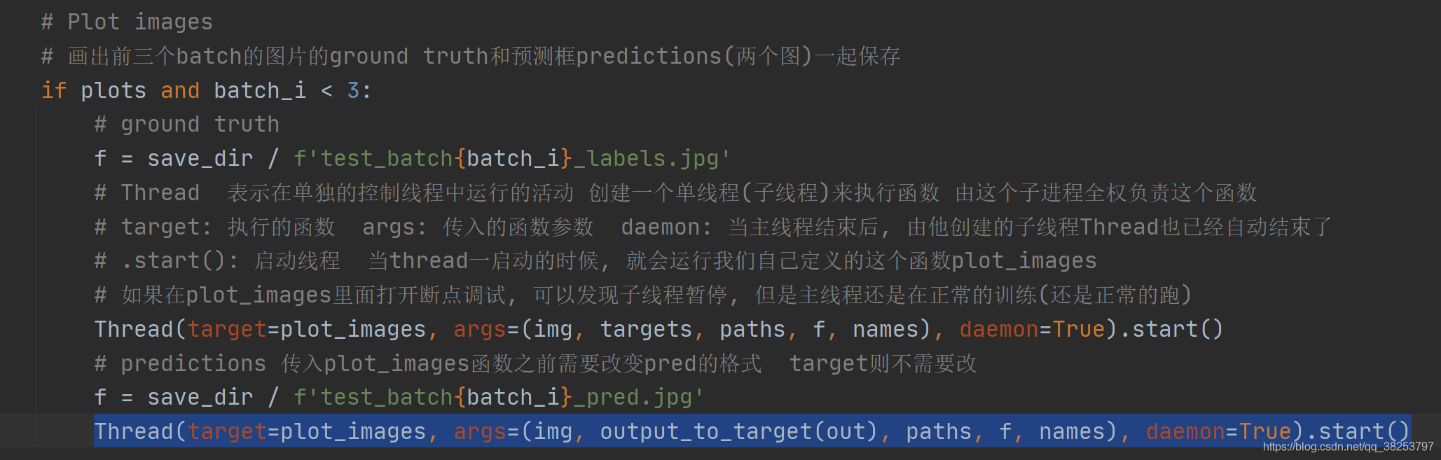
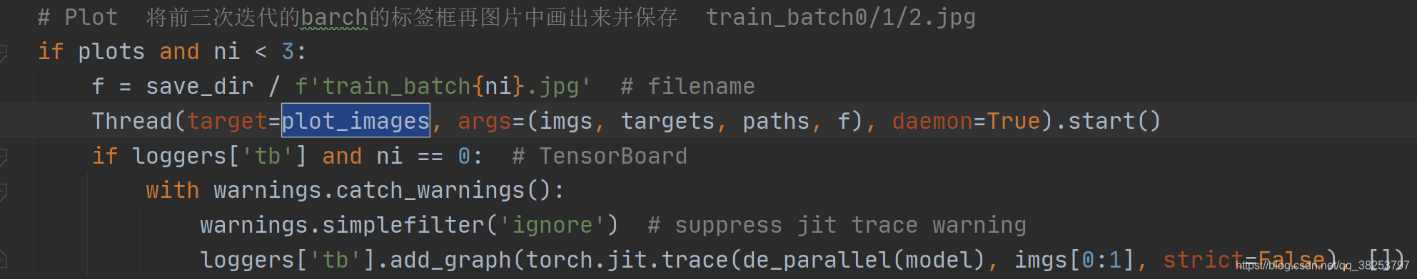
\qquad�����������������һ��batch������ͼƬ�Ŀ����ʵ���Ԥ���ʹ����test.py�У�����output_to_target����֮������������ǽ�һ��batch��ͼƬ������һ����ͼmosaic���棬�Ų���ɾ����
plot_images��������:
def plot_images(images, targets, paths=None, fname='images.jpg', names=None, max_size=640, max_subplots=16):"""����test.py�н��л���ǰ3��batch��ground truth��Ԥ���predictions(����ͼ) һ�𱣴� ����train.py�н�����batch��labels���������batch��images��Plot image grid with labels:params images: ��ǰbatch������ͼƬ Tensor [batch_size, 3, h, w] ��ͼƬ���ǹ�һ�����:params targets: ֱ������target: Tensor[num_target, img_index+class+xywh] [num_target, 6]����output_to_target: Tensor[num_pred, batch_id+class+xywh+conf] [num_pred, 7]:params paths: tuple ��ǰbatch������ͼƬ�ĵ�ַ��: '..\\datasets\\coco128\\images\\train2017\\000000000315.jpg':params fname: ���ձ�����ļ�·�� + ���� runs\train\exp8\train_batch2.jpg:params names: ��������� ��class index������Ӧ��keyֵ ����Ĭ����None ֻ��ʾclass index����ʾ����:params max_size: ͼƬ�����ߴ�640 ���images��ͼƬ�Ĵ�С(w/h)����640����Ҫresize �������С��640����Ҫresize:params max_subplots: �����ͼ���� 16:params mosaic: һ�Ŵ�ͼ ��������ʾmax_subplots��ͼƬ ���ܶ��ͼƬ(�������Ե�label���)һ������һ����ʾmosaicÿ��ͼƬ�����Ϸ�������ʾ��ǰͼƬ������ �����fnameΪ����������"""if isinstance(images, torch.Tensor):images = images.cpu().float().numpy() # tensor -> numpy arrayif isinstance(targets, torch.Tensor):targets = targets.cpu().numpy()# ����һ�� ����һ�����ͼƬ��ԭ un-normaliseif np.max(images[0]) <= 1:images *= 255# ����һЩ��������tl = 3 # �����߿� line thickness 3tf = max(tl - 1, 1) # ��������ʻ��߿� font thickness 2bs, _, h, w = images.shape # batch size 4, channel 3, height 512, width 512bs = min(bs, max_subplots) # ��ͼ���� ������ limit plot images 4ns = np.ceil(bs ** 0.5) # ns=ÿ��/ÿ�������ͼ���� ��ͼ����=ns*ns ceil����ȡ�� 2# Check if we should resize# ���images��ͼƬ�Ĵ�С(w/h)����640����Ҫresize �������С��640����Ҫresizescale_factor = max_size / max(h, w) # 1.25if scale_factor < 1:# ���w/h���κ�һ���߳���640, ��Ҫ���ϳ������ŵ�640, ����һ������ӦҲ����h = math.ceil(scale_factor * h) # 512w = math.ceil(scale_factor * w) # 512# np.full ����һ��ָ����״�����ͺ���ֵ������# shape: (int(ns * h), int(ns * w), 3) (1024, 1024, 3) ����ֵ: 255 dtype �������: np.uint8mosaic = np.full((int(ns * h), int(ns * w), 3), 255, dtype=np.uint8) # init# ��batch��ÿ��ͼƬfor i, img in enumerate(images): # img (3, 512, 512)# ���ͼƬҪ����max_subplots���ǾͲ�����if i == max_subplots: # if last batch has fewer images than we expectbreak# (block_x, block_y) �൱�������Ͻǵ����block_x = int(w * (i // ns)) # // ȡ�� 0 0 512 512 ns=2block_y = int(h * (i % ns)) # % ȡ�� 0 512 0 512img = img.transpose(1, 2, 0) # (512, 512, 3) h w cif scale_factor < 1: # ���scale_factor < 1˵��h/w����max_size ��Ҫresize����img = cv2.resize(img, (w, h))# �����batch��ͼƬһ���ŵ�����mosaic��Ӧ��λ���� hwc ��������Լ�����ͼ������# ��һ��ͼmosaic[0:512, 0:512, :] �ڶ���ͼmosaic[512:1024, 0:512, :]# ������ͼmosaic[0:512, 512:1024, :] ������ͼmosaic[512:1024, 512:1024, :]mosaic[block_y:block_y + h, block_x:block_x + w, :] = imgif len(targets) > 0:# �����������img��targetimage_targets = targets[targets[:, 0] == i]# ������ͼƬ������target��xywh -> xyxyboxes = xywh2xyxy(image_targets[:, 2:6]).T# �õ�����ͼƬ����target�����classesclasses = image_targets[:, 1].astype('int')# ���image_targets.shape[1] == 6��˵��û�����Ŷ���Ϣ(��ʱtargetʵ��������ʵ��)# �������Ϊ7���7����Ϣ�������Ŷ���Ϣ(��ʱtargetΪԤ�����Ϣ)labels = image_targets.shape[1] == 6 # labels if no conf column# �õ���ǰ����ͼ������target�����Ŷ���Ϣ(pred) ���û�о�Ϊ��(��ʵlabel)# check for confidence presence (label vs pred)conf = None if labels else image_targets[:, 6]if boxes.shape[1]: # boxes.shape[1]��Ϊ��˵������ͼ��targetĿ��if boxes.max() <= 1.01: # if normalized with tolerance 0.01# ��ΪͼƬ�Ƿ���һ���� ��������boxesҲ����һ��boxes[[0, 2]] *= w # scale to pixelsboxes[[1, 3]] *= helif scale_factor < 1:# ���scale_factor < 1 ˵��resize��, ��ôboxesҲҪ��Ӧ�仯# absolute coords need scale if image scalesboxes *= scale_factor# ����õ���boxes��Ϣ�����img����ͼƬ�ı�ǩ��Ϣ ��Ϊ����������Ҫ��img����mosaic�� ���Ի�Ҫ�任label->mosaicboxes[[0, 2]] += block_xboxes[[1, 3]] += block_y# ����ǰ��ͼƬimg�����б�ǩboxes����mosaic��for j, box in enumerate(boxes.T):# ����ÿ��boxcls = int(classes[j]) # �õ����box��class indexcolor = colors(cls) # �õ����box���ߵ���ɫcls = names[cls] if names else cls # ���������������ʾ���� ���û������������ʾclass index# ���labels��Ϊ��˵��������ʾ��ʵtarget ����Ҫconf���Ŷ� ֱ����ʾlabel����# ���conf[j] > 0.25 ����˵��������ʾpred �����box��conf�������0.25 �൱������һ��nmsɸѡ ��ʾlabel + confif labels or conf[j] > 0.25: # 0.25 conf threshlabel = '%s' % cls if labels else '%s %.1f' % (cls, conf[j]) # ����������ʾ��Ϣplot_one_box(box, mosaic, label=label, color=color, line_thickness=tl) # һ�����Ļ���# ��mosaicÿ��ͼƬ���λ�õ����Ͻ�д��ÿ��ͼƬ���ļ��� ��000000000315.jpgif paths:# paths[i]: '..\\datasets\\coco128\\images\\train2017\\000000000315.jpg' Path: str -> Wins��ַ# .name: str'000000000315.jpg' [:40]ȡǰ40���ַ� ���ջ��ǵ���str'000000000315.jpg'label = Path(paths[i]).name[:40] # trim to 40 char# �����ı� label �Ŀ��� (width, height)t_size = cv2.getTextSize(label, 0, fontScale=tl / 3, thickness=tf)[0]# ��mosaic��д�ı���Ϣ# Ҫ���Ƶ�ͼ�� + Ҫд��ǰ���ı���Ϣ + �ı����½����� + Ҫʹ�õ����� + ��������ϵ�� + �������ɫ + ������߿� + ���α߿������cv2.putText(mosaic, label, (block_x + 5, block_y + t_size[1] + 5), 0,tl / 3, [220, 220, 220], thickness=tf, lineType=cv2.LINE_AA)# mosaic��ÿ��ͼƬ��ͼƬ֮��Ūһ���߽����� �ÿ��� ��ʵ�����ؼ� ���ǽ�ÿ��img��mosaic�л�����cv2.rectangle(mosaic, (block_x, block_y), (block_x + w, block_y + h), (255, 255, 255), thickness=3)# ���һ�� check�Ƿ���Ҫ��mosaicͼƬ��������if fname: # �ļ�����Ϊ�յĻ� fname = runs\train\exp8\train_batch2.jpg# ����mosaicͼƬ�ߴ�r = min(1280. / max(h, w) / ns, 1.0) # ratio to limit image sizemosaic = cv2.resize(mosaic, (int(ns * w * r), int(ns * h * r)), interpolation=cv2.INTER_AREA)# cv2.imwrite(fname, cv2.cvtColor(mosaic, cv2.COLOR_BGR2RGB)) # cv2 save ���BGR -> RGB�ٱ���Image.fromarray(mosaic).save(fname) # PIL save ����Ҫnumpy array -> tensor��ʽ ���ܱ���return mosaic
������������������test.py�����еģ�
����train.py��
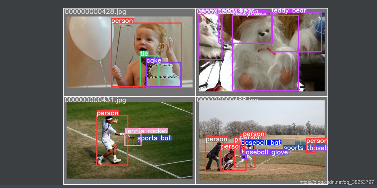
ִ��Ч��test.py��target����
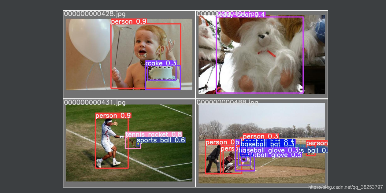
 ִ��Ч��test.py��predict����
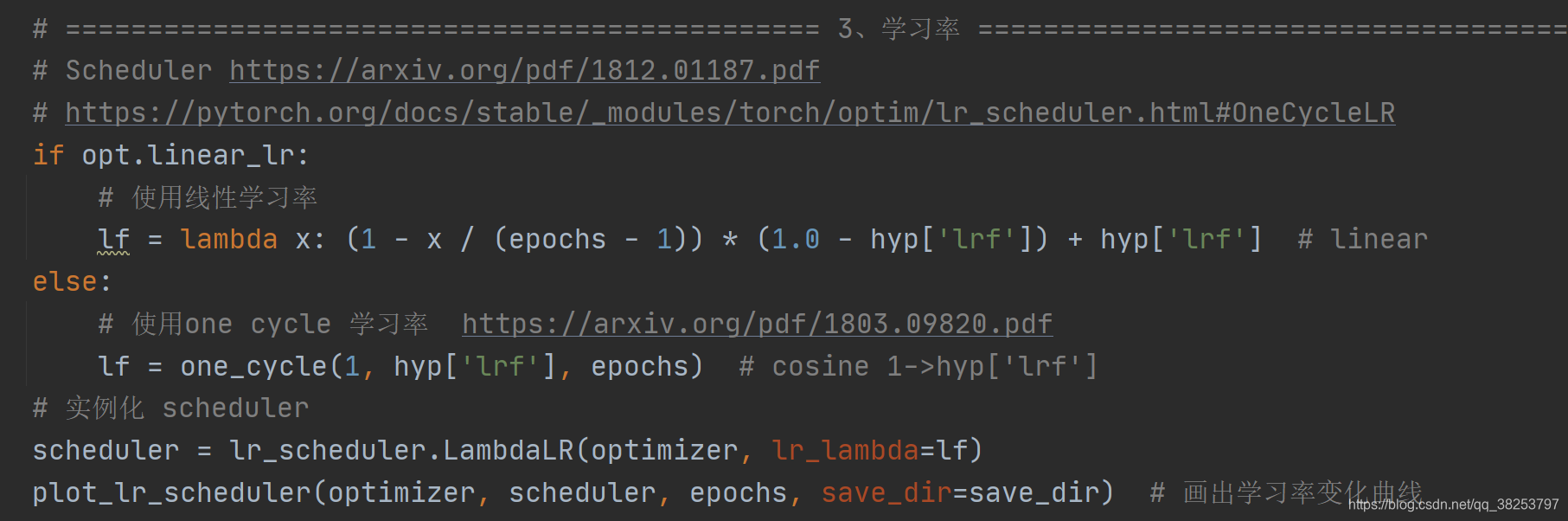
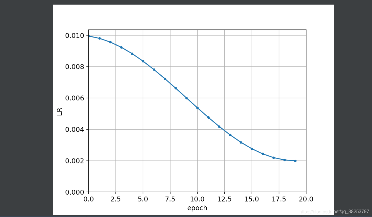
5��plot_lr_scheduler
\qquad�������������������ѵ��������ÿ��epoch��ѧϰ�ʱ仯�����
plot_lr_scheduler�������룺
def plot_lr_scheduler(optimizer, scheduler, epochs=300, save_dir=''):"""����train.py��ѧϰ�����ú���ӻ�һ��Plot LR simulating training for full epochs:params optimizer: �Ż���:params scheduler: ���Ե�����:params epochs: x:params save_dir: lrͼƬ �����ַ"""optimizer, scheduler = copy(optimizer), copy(scheduler) # do not modify originalsy = [] # ���ÿ��epoch��ѧϰ��# ��optimizer��ȡѧϰ�� һ��epochȡһ�� ��ȡepochs�� ÿȡһ����Ҫʹ��scheduler.step������һ��epoch��ѧϰ��for _ in range(epochs):scheduler.step() # ������һ��epoch��ѧϰ��# ptimizer.param_groups[0]['lr']: ȡ��һ��epoch��ѧϰ��lry.append(optimizer.param_groups[0]['lr'])plt.plot(y, '.-', label='LR') # û�д���x Ĭ�ϻᴫ�� 0..epochs-1plt.xlabel('epoch')plt.ylabel('LR')plt.grid()plt.xlim(0, epochs)plt.ylim(0)plt.savefig(Path(save_dir) / 'LR.png', dpi=200) # ����plt.close()
ͨ������train.py��ѧϰ�����ú���ӻ�һ�£�
ִ��Ч����
6��hist2d��plot_test_txt��plot_targets_txt
6.1��hist2d
\qquad���������ʹ��numpy������2dֱ��ͼ�����������õIJ��࣬��������ǵ��ù��߰���װ�õ�2dֱ��ͼ�����������������ʵֻ��plot_evolution������plot_test_txt������ʹ�á�
hist2d�������룺
def hist2d(x, y, n=100):"""����plot_evolution��plot_test_txtʹ��numpy����2dֱ��ͼ2d histogram used in labels.png and evolve.png"""# xedges: ������start=x.min()��stop=x.max()֮�䷵�ؾ��ȼ����n������xedges, yedges = np.linspace(x.min(), x.max(), n), np.linspace(y.min(), y.max(), n)# np.histogram2d: 2dֱ��ͼ x: x������ y: y������ (xedges, yedges): bins x, y��ij�������Ŀ# ����hist: ֱ��ͼ���� xedges: x����� yedges: y�����hist, xedges, yedges = np.histogram2d(x, y, (xedges, yedges))# np.clip: ��ȡ���� ��Ŀ�����������ݶ�����һ����Χ [0, hist.shape[0] - 1] С��0�ĵ���0 ����ͬ��# np.digitize ���ڷ���xidx = np.clip(np.digitize(x, xedges) - 1, 0, hist.shape[0] - 1) # x������yidx = np.clip(np.digitize(y, yedges) - 1, 0, hist.shape[1] - 1) # y������return np.log(hist[xidx, yidx])
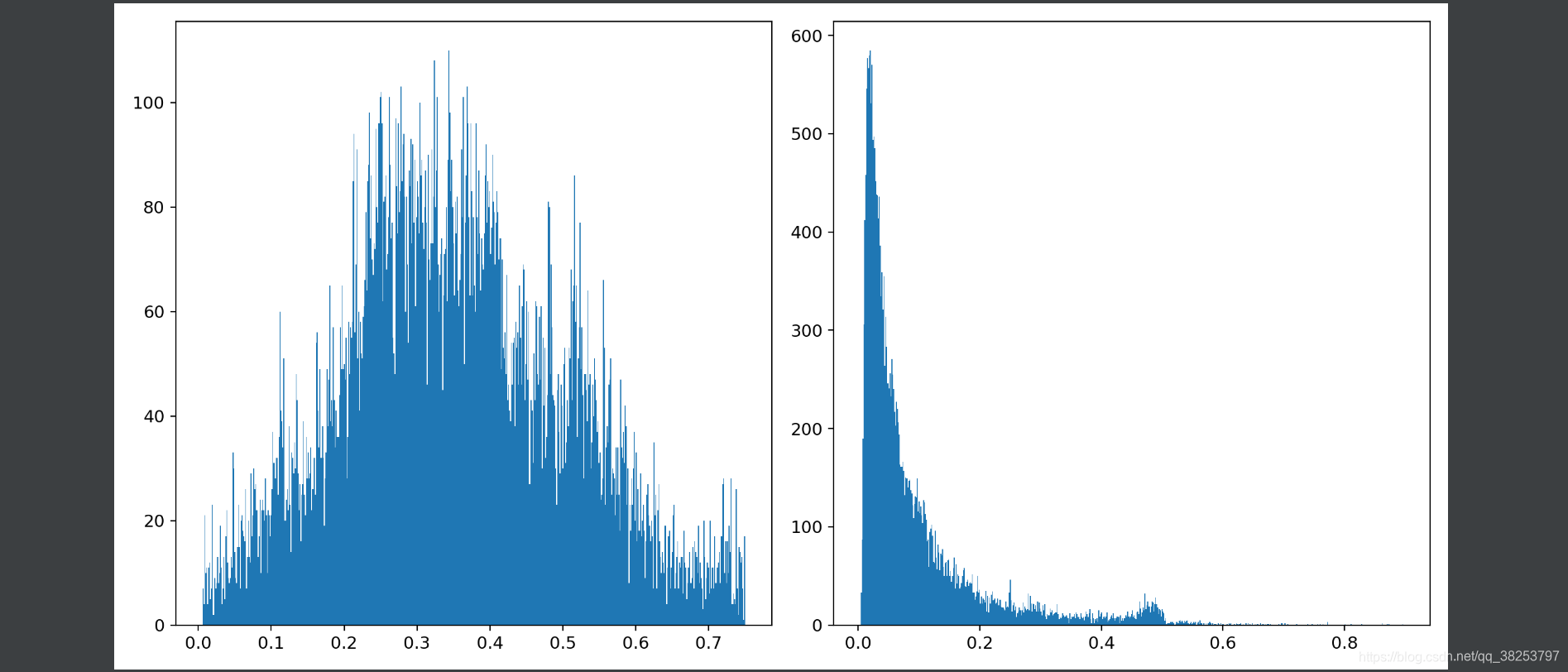
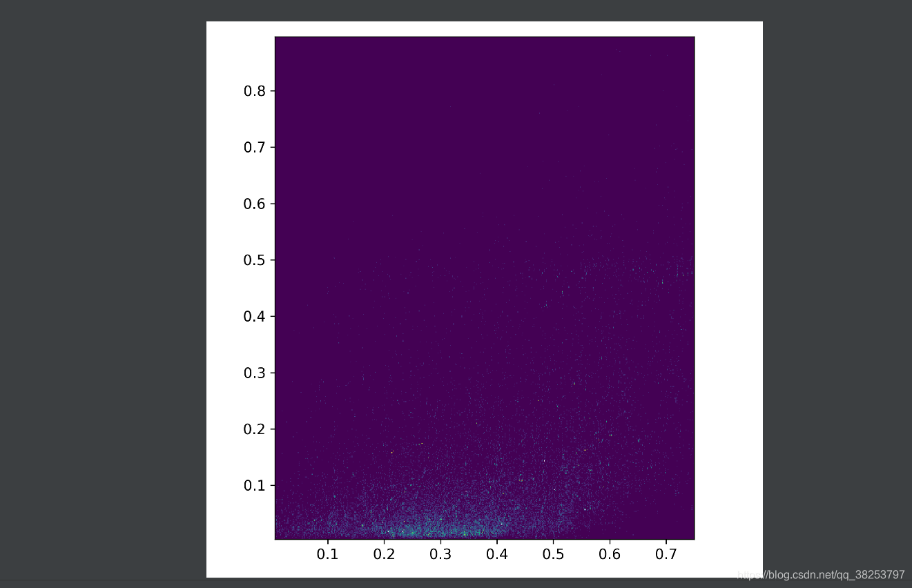
6.2��plot_test_txt
\qquad�������������test.py�����ɵ�test.txt�ļ�������������*.txt�ļ�����������xyֱ��ͼ��xy˫ֱ��ͼ����ʵ���plot_test_txt����������߲�û��ʹ��������������ȷʵ�����Լ�дһ���ű���ִ������������۲�һ��Ԥ�������ͼ���Ŀ�������wh�ֲ�����
plot_test_txt�������룺
def plot_test_txt(test_dir='test.txt'):"""�����Լ�д���ű�ִ��test.txt�ļ�����test.txt xyxy������ֱ��ͼ��˫ֱ��ͼPlot test.txt histograms:params test_dir: test.py�����ɵ�һЩ save_dir/labels�е�txt�ļ�"""# x [:, xyxy]x = np.loadtxt(test_dir, dtype=np.float32)box = xyxy2xywh(x[:, 2:6]) # xyxy to xywh �����Ҹ����� ԭ����0:4 ���ҷ���txt�д�ŵ��� cls+conf+xyxycx, cy = box[:, 0], box[:, 1] # x y# ��figure�ֳ�1��1�� figure size=(6, 6) tight_layout=true ���Զ�������ͼ����, ʹ֮�������ͼ������# ����figure(��ͼ����)��axes(�������)fig, ax = plt.subplots(1, 1, figsize=(6, 6), tight_layout=True)# hist2d: ˫ֱ��ͼ cx: x���� cy: y���� bins: ������Ϊ���� cmax��cmin: ���е�bins��ֵ����cmin�ʹ���cmax�IJ���ʾax.hist2d(cx, cy, bins=600, cmax=10, cmin=0)ax.set_aspect('equal') # ����������ij���ʼ����ͬ figureΪ������plt.savefig('hist2d.png', dpi=300)fig, ax = plt.subplots(1, 2, figsize=(12, 6), tight_layout=True)# hist ����ֱ��ͼ cx: ��ͼ���� bins: ֱ��ͼ�ij�������Ŀ normed: �Ƿõ���ֱ��ͼ������һ��# facecolor: �����ε���ɫ edgecolor:�����α߿����ɫ alpha:����ax[0].hist(cx, bins=600)ax[1].hist(cy, bins=600)plt.savefig('hist1d.png', dpi=200)
�Լ�д���ű�ʹ�ã�

hist1d.pngЧ����������ֱ���w��h���������Ǹ�������
hist2d.png������������x��������y����
6.3��plot_targets_txt��û�õ���
\qquad�������������targets.txt����ʵ���xywh��������ֱ��ͼ�����Dz�û��ʹ���������������ϸ�ĵĿ��Է������������֮���plot_labels�������ظ��ġ����������������㿴���ɡ�
plot_targets_txt�������룺
def plot_targets_txt():"""û�õ� ��plot_labels�����ظ�����targets.txt xywh������ֱ��ͼPlot targets.txt histograms"""# x [:, xywh]x = np.loadtxt('targets.txt', dtype=np.float32).Ts = ['x targets', 'y targets', 'width targets', 'height targets']fig, ax = plt.subplots(2, 2, figsize=(8, 8), tight_layout=True)ax = ax.ravel() # ����ά���齵λһάfor i in range(4):ax[i].hist(x[i], bins=100, label='%.3g +/- %.3g' % (x[i].mean(), x[i].std()))ax[i].legend() # ��ʾ����labelͼ��ax[i].set_title(s[i])plt.savefig('targets.jpg', dpi=200)
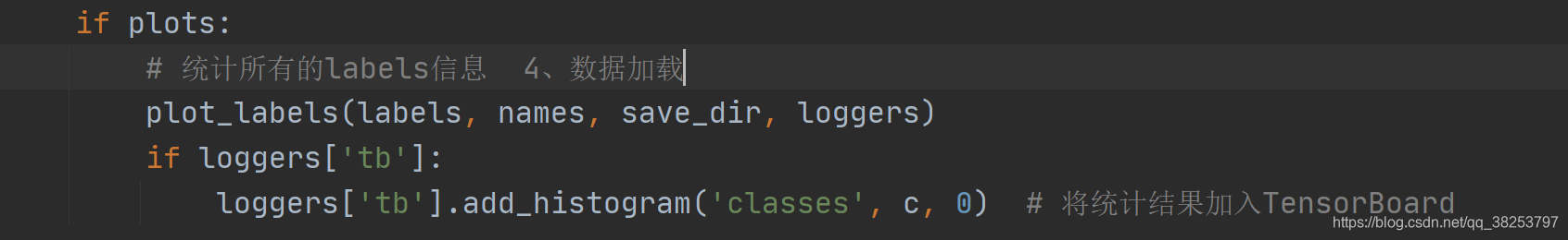
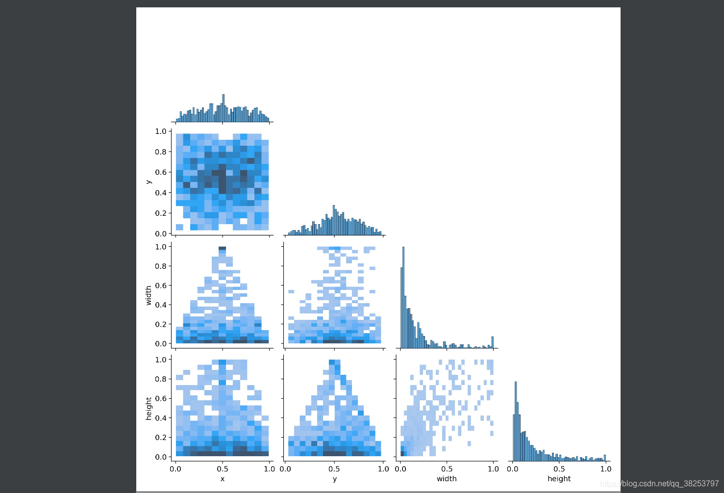
7��plot_labels
\qquad��������Ǹ��ݴ�datasets��ȡ����labels�����������ֲ�������labels���ֱ��ͼ��Ϣ�����ջ�����labels_correlogram.jpg��labels.jpg����ͼƬ��labels_correlogram.jpg�������б�ǩ�� x��y��w��h�Ķ�������Ϸֲ�ֱ��ͼ���鿴�������������ϱ���֮���������ϵ�Ŀ��ӻ���ʽ���������x��y��w��h����֮��ķֲ�ֱ��ͼ������labels.jpg�����ˣ�ax[0]����classes�ĸ�����ķֲ�ֱ��ͼ��ax[1]�������е���ʵ��ax[2]����xyֱ��ͼ��ax[3]����whֱ��ͼ��
plot_labels�������룺
def plot_labels(labels, names=(), save_dir=Path(''), loggers=None):"""ͨ������train.py�� ��������datasets��labels�� ��labels���п��ӻ� ����labels��Ϣplot dataset labels ����labels_correlogram.jpg��labels.jpg �������ݼ���labels���ֱ��ͼ��Ϣ:params labels: ���ݼ���ȫ����ʵ���ǩ (num_targets, class+xywh) (929, 5):params names: ���ݼ������������:params save_dir: runs\train\exp21:params loggers: ��־����"""print('Plotting labels... ')# c: classes (929) b: boxes xywh (4, 929) .transpose() ��(4, 929) -> (929, 4)c, b = labels[:, 0], labels[:, 1:].transpose()nc = int(c.max() + 1) # ������� number of classes 80# pd.DataFrame: ����DataFrame, ������һ��excel, ��ͷ��['x', 'y', 'width', 'height'] ��������: b�����ݰ������δ洢x = pd.DataFrame(b.transpose(), columns=['x', 'y', 'width', 'height'])# 1������labels�� xywh �������Ϸֲ�ֱ��ͼ labels_correlogram.jpg# seaborn correlogram seaborn.pairplot ��������Ϸֲ�ͼ: �鿴�������������ϱ���֮���������ϵ�Ŀ��ӻ���ʽ# data: ���Ϸֲ�����x diag_kind:��ʾ���Ϸֲ�ͼ�жԽ���ͼ������ kind:��ʾ���Ϸֲ�ͼ�зǶԽ���ͼ������# corner: True ��ʾֻ��ʾ���²� ��Ϊ���º��������ظ��� plot_kws,diag_kws: ���Խ����ֵ�IJ�������ͼ�ν�����sn.pairplot(x, corner=True, diag_kind='auto', kind='hist', diag_kws=dict(bins=50), plot_kws=dict(pmax=0.9))plt.savefig(save_dir / 'labels_correlogram.jpg', dpi=200) # ����labels_correlogram.jpgplt.close()# 2������classes�ĸ�����ķֲ�ֱ��ͼax[0], �������е���ʵ��ax[1], ����xyֱ��ͼax[2], ����whֱ��ͼax[3] labels.jpgmatplotlib.use('svg') # faster# ������figure�ֳ�2*2�ĸ�����ax = plt.subplots(2, 2, figsize=(8, 8), tight_layout=True)[1].ravel()# ��һ������ax[1]����classes�ķֲ�ֱ��ͼy = ax[0].hist(c, bins=np.linspace(0, nc, nc + 1) - 0.5, rwidth=0.8)# [y[2].patches[i].set_color([x / 255 for x in colors(i)]) for i in range(nc)] # update colors bug #3195ax[0].set_ylabel('instances') # ����y��labelif 0 < len(names) < 30: # С��30�����Ͱ����е��������Ϊ������ax[0].set_xticks(range(len(names))) # ���ÿ̶�ax[0].set_xticklabels(names, rotation=90, fontsize=10) # ��ת90�� ����ÿ���̶ȱ�ǩelse:ax[0].set_xlabel('classes') # ������������30��, ���ܾͷŲ���ȥ��, ����ֻ��ʾx��label# ����������ax[2]����xyֱ��ͼ ���ĸ�����ax[3]����whֱ��ͼsn.histplot(x, x='x', y='y', ax=ax[2], bins=50, pmax=0.9)sn.histplot(x, x='width', y='height', ax=ax[3], bins=50, pmax=0.9)# �ڶ�������ax[1]�������е���ʵ��labels[:, 1:3] = 0.5 # center xylabels[:, 1:] = xywh2xyxy(labels[:, 1:]) * 2000 # xyxyimg = Image.fromarray(np.ones((2000, 2000, 3), dtype=np.uint8) * 255) # ��ʼ��һ������for cls, *box in labels[:1000]: # �����еĿ���img������ImageDraw.Draw(img).rectangle(box, width=1, outline=colors(cls)) # plotax[1].imshow(img)ax[1].axis('off') # ��Ҫxy��# ȥ��������������ϵ(ȥ���������ұ߿�)for a in [0, 1, 2, 3]:for s in ['top', 'right', 'left', 'bottom']:ax[a].spines[s].set_visible(False)plt.savefig(save_dir / 'labels.jpg', dpi=200)matplotlib.use('Agg')plt.close()# ��ӡ��־ loggersfor k, v in loggers.items() or {
}:if k == 'wandb' and v:v.log({
"Labels": [v.Image(str(x), caption=x.name) for x in save_dir.glob('*labels*.jpg')]}, commit=False)
�������һ�������train.py����������datasets��labels��ͳ�Ʒ���labels��طֲ���Ϣ��
labels_correlogram.jpgִ��Ч����
labels.jpgִ��Ч����
8��plot_evolution
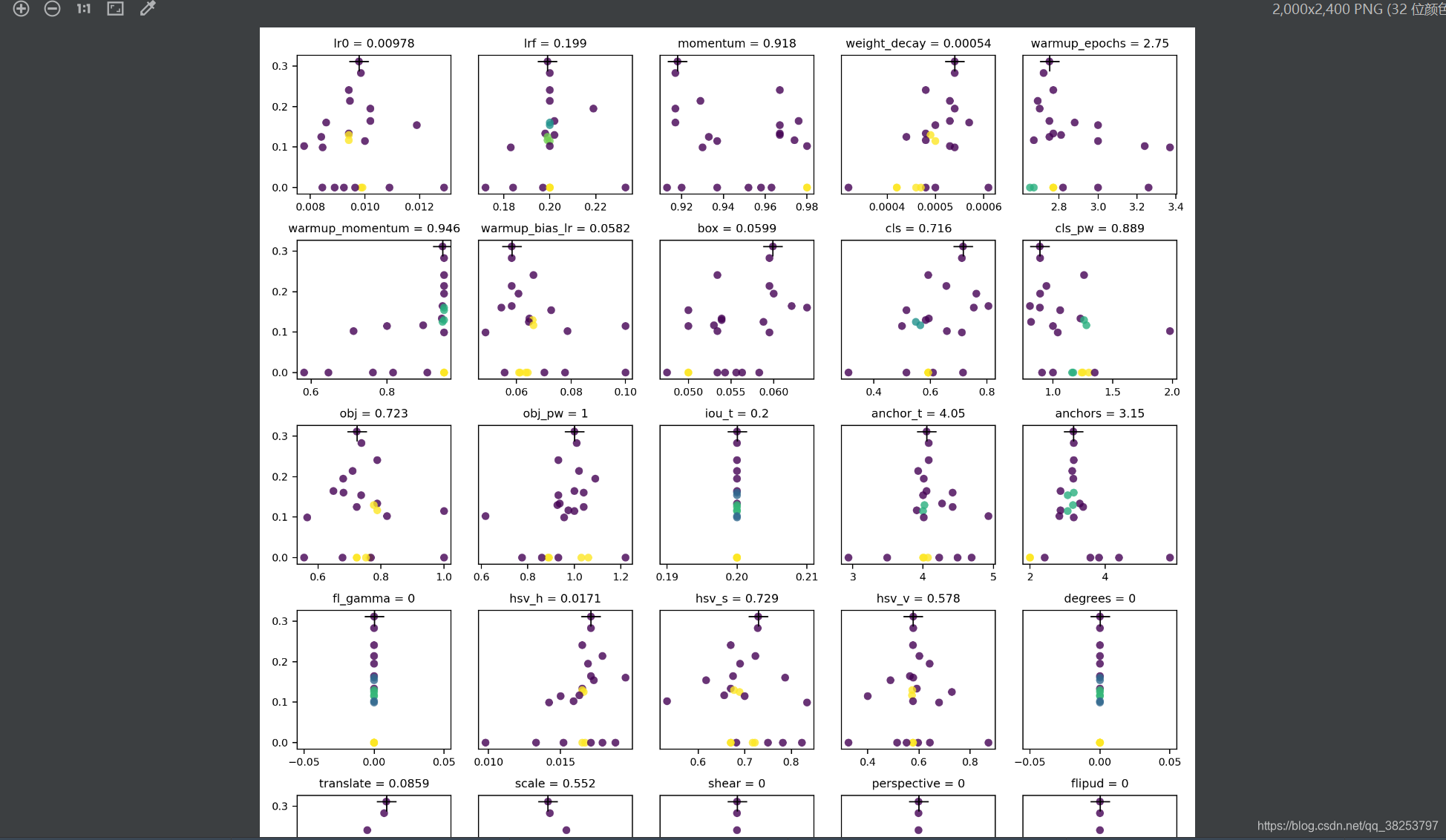
\qquad����������ڳ��ν��������Σ�����ÿ�����ν����Ľ�������ջ�����evolve.png��������ÿ�����εĽ�������Լ����Ӧ��mAP��ɢ��ͼ��ÿ5������һ�У����һ��� ��+�� ��ע�����mAP��Ӧ�ij���ֵ����ÿ��ɢ��ͼ��������mAP��Ӧ��ÿ�����ε���ѳ��Ρ�����plot_evolutionҲ�����������hist2d������
plot_evolution�������룺
def plot_evolution(yaml_file='data/hyp.finetune.yaml', save_dir=Path('')):"""����train.py�ij��ν����㷨������γ������Ľ�����ν�����ÿһ�ֶ������һϵ�еĽ�����ij���(����yaml_file) �Լ�ÿһ�ֶ��������ǰ�ִε�7��ָ��(evolve.txt)�������Ҫ���ľ��ǰ�ÿ�������������ִα仯��ֵ��maps��ɢ��ͼ����ʽ��ʾ����,���������map��Ӧ�ij���ֵ һ������һ��ɢ��ͼ:params yaml_file: 'runs/train/evolve/hyp_evolved.yaml'"""with open(yaml_file) as f:hyp = yaml.safe_load(f) # ���볬���ļ�# evolve.txt��ÿһ��Ϊһ�ν����Ľ��# ÿ��ǰ�߸�����(P, R, mAP, F1, test_losses(GIOU, obj, cls)) ֮��Ϊhypx = np.loadtxt('evolve.txt', ndmin=2)f = fitness(x) # �õ����н����ִκ�õ��ļ�Ȩ��ʽ��map# weights = (f - f.min()) ** 2 # for weighted resultsplt.figure(figsize=(10, 12), tight_layout=True)matplotlib.rc('font', **{
'size': 8}) # ����matplotlib���� font_size: 8for i, (k, v) in enumerate(hyp.items()):y = x[:, i + 7] # y=��ǰ������ÿһ�ֽ������ֵ# mu = (y * weights).sum() / weights.sum() # best weighted resultmu = y[f.argmax()] # �õ���Ȩmap����epochʱ�ij���(��Ϊ�������Ϊ�����ִε���ѳ���)plt.subplot(6, 5, i + 1) # ������30������ 6��5�� һ�����ֻ�һ��ͼ# ����ÿ�����α仯��ɢ��ͼ x: x����Ϊ��ǰ����ÿһ�ֽ������ֵy y: y����Ϊ���н����ִκ�õ��ļ�Ȩ��ʽ��map# c: ɫ�ʻ���ɫ cmap: Colormapʵ�� alpha: edgecolors: �߿���ɫplt.scatter(y, f, c=hist2d(y, f, 20), cmap='viridis', alpha=.8, edgecolors='none')# �ڵ�ǰСͼ���ٻ������mapʱ��Ӧ�ij��� ���� '+' ���Ǻ�plt.plot(mu, f.max(), 'k+', markersize=15)plt.title('%s = %.3g' % (k, mu), fontdict={
'size': 9}) # limit to 40 charactersif i % 5 != 0: # һ��ֻ�ܻ�5��Сͼplt.yticks([])print('%15s: %.3g' % (k, mu)) # �����ѳ���plt.savefig(save_dir / 'evolve.png', dpi=200) # ����evolve.pngprint('\nPlot saved as evolve.png')
�������ͨ��������train.py�ij��ν����㷨������γ������Ľ����
����ִ��Ч��evolve.png:
9��plot_results��plot_results_overlay��butter_lowpass_filtfilt
\qquad��������������������result.txt�еĸ���ָ����п��ӻ��ģ�����plot_results�ǽ�һ��ָ�껭������ͼ�ϣ���10������ͼ������ plot_results_overlayҪ�����ǽ�ԭ�ȵ�10����ʾ��ָ�꣬�����������жԱȻ���ͬһ������ͼ�ϣ���5������ͼ��������butter_lowpass_filtfilt����
9.1��plot_results
\qquad��������ǽ�ѵ����Ľ�� results.txt ����ص�ѵ��ָ�껭������
\qquadresult.txt��һ�е�Ԫ�طֱ��У���ǰepoch/��epochs-1 ����ǰ���Դ�����mem��box�ع���ʧ��obj���Ŷ���ʧ��cls������ʧ��ѵ������ʧ����ʵĿ������num_target��ͼƬ�ߴ�img_shape��Precision��Recall��map@0.5��map@0.5:0.95������box�ع���ʧ������obj���Ŷ��𡢲���cls������ʧ��
\qquad��result.txt�л�����ָ���У�ѵ���ع���ʧBox��ѵ�����Ŷ���ʧObjectness��ѵ��������ʧClassification��Precision��Recall����֤�ع���ʧ val Box����֤���Ŷ���ʧval Objectness����֤������ʧval Classification��mAP@0.5��mAP@0.5:0.95��
plot_results�������룺
def plot_results(start=0, stop=0, bucket='', id=(), save_dir=''):"""'����ѵ������, ��ѵ��������п��ӻ�����ѵ����� results.txt Plot training 'results*.txt' ��������results.png:params start: ��ȡ���ݵĿ�ʼepoch ��Ϊresult.txt��������һ��epochһ�е�:params stop: ��ȡ���ݵĽ���epoch:params bucket: �Ƿ���Ҫ��googleapis������results*.txt�ļ�:params id: ��Ҫ��googleapis�����ص�results + id.txt Ĭ��Ϊ��:params save_dir: 'runs\train\exp22'"""# ����һ��figure �ָ��2��5��, ��10��Сsubplots���fig, ax = plt.subplots(2, 5, figsize=(12, 6), tight_layout=True)ax = ax.ravel() # ����ά���齵Ϊһάs = ['Box', 'Objectness', 'Classification', 'Precision', 'Recall','val Box', 'val Objectness', 'val Classification', 'mAP@0.5', 'mAP@0.5:0.95'] # titlesif bucket:# files = ['https://storage.googleapis.com/%s/results%g.txt' % (bucket, x) for x in id]files = ['results%g.txt' % x for x in id]c = ('gsutil cp ' + '%s ' * len(files) + '.') % tuple('gs://%s/results%g.txt' % (bucket, x) for x in id) # cmdָ��os.system(c) # ʹ��cmdָ���googleapis������results*.txtelse:# �������������ؾ�ֱ�Ӵ��ļ�Ŀ¼��ģ������ ��files=[WindowsPath('runs/train/exp22/results.txt')]files = list(Path(save_dir).glob('results*.txt')) # ����save_dirĿ¼������'results*.txt'�ļ������ļ�assert len(files), 'No results.txt files found in %s, nothing to plot.' % os.path.abspath(save_dir)# ��ȡfiles�ļ����ݽ��п��ӻ�for fi, f in enumerate(files):try:# files ԭʼһ��: epoch/epochs - 1, memory, Box, Objectness, Classification, sum_loss, targets.shape[0], img_shape, Precision, Recall, map@0.5, map@0.5:0.95, Val Box, Val Objectness, Val Classification# ֻʹ��[2, 3, 4, 8, 9, 12, 13, 14, 10, 11]�� (10, 1) �ֲ���Ӧ =># [Box, Objectness, Classification, Precision, Recall, Val Box, Val Objectness, Val Classification, map@0.5, map@0.5:0.95]results = np.loadtxt(f, usecols=[2, 3, 4, 8, 9, 12, 13, 14, 10, 11], ndmin=2).T # (10, 1)n = results.shape[1] # number of rows 1# ����start(epoch)��stop(epoch)��ȡ��Ӧ���ִε�����x = range(start, min(stop, n) if stop else n)for i in range(10): # �ֱ���ӻ���10��ָ��y = results[i, x]if i in [0, 1, 2, 5, 6, 7]:y[y == 0] = np.nan # lossֵ����Ϊ0 Ҫ��ʾΪnp.nan# y /= y[0] # normalize# label = labels[fi] if len(labels) else f.stemax[i].plot(x, y, marker='.', linewidth=2, markersize=8) # ����ͼ# ax[i].plot(x, y, marker='.', label=label, linewidth=2, markersize=8)ax[i].set_title(s[i]) # ������ͼ����# if i in [5, 6, 7]: # share train and val loss y axes# ax[i].get_shared_y_axes().join(ax[i], ax[i - 5])except Exception as e:print('Warning: Plotting error for %s; %s' % (f, e))# ax[1].legend()fig.savefig(Path(save_dir) / 'results1.png', dpi=200) # ����results.png
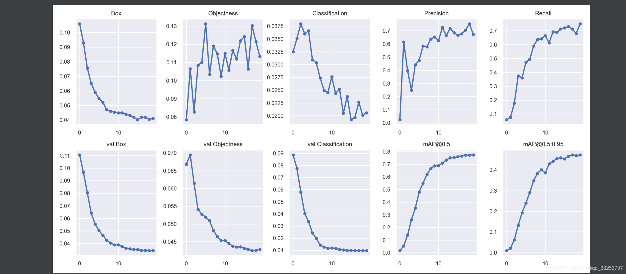
�������������train.pyѵ���������ѵ��������п��ӻ���
ִ�н��result1.png��
9.2��plot_results_overlay
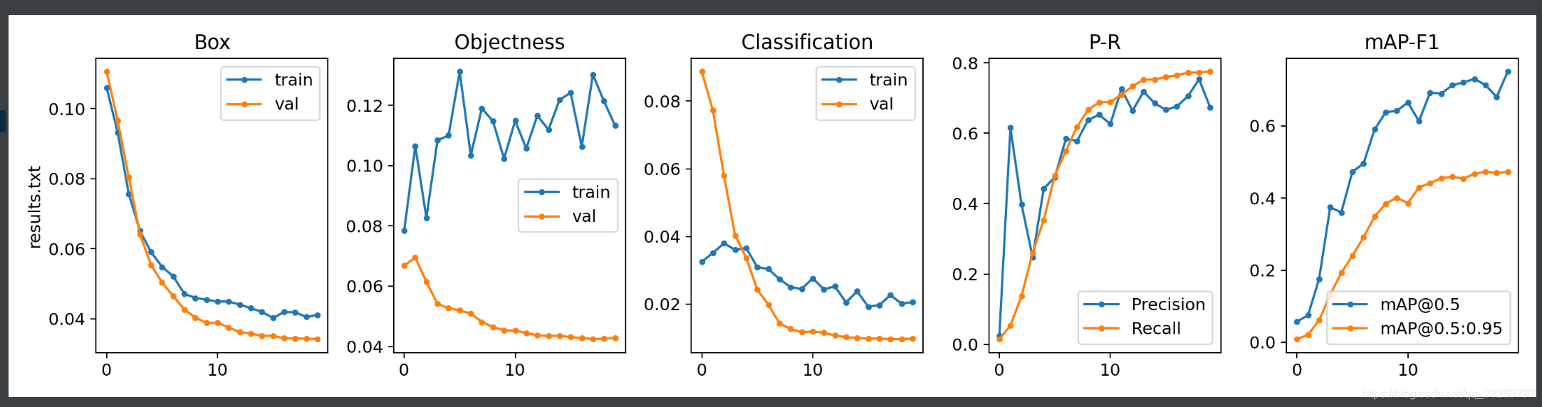
\qquad����������ǽ�result.txt�ļ��еĸ���ָ����п��ӻ���������ԭ�ȵ�10������ͼ��Ϊ5������ͼ, train��val������Աȡ�
plot_results_overlay�������룺
def plot_results_overlay(start=0, stop=0):"""��������train.py������дһ���ļ�����ѵ����� results.txt Plot training 'results*.txt' ���ҽ�ԭ�ȵ�10������ͼ����Ϊ5������ͼ, train��val��Ա�Plot training 'results*.txt', overlaying train and val losses"""s = ['train', 'train', 'train', 'Precision', 'mAP@0.5', 'val', 'val', 'val', 'Recall', 'mAP@0.5:0.95'] # legendst = ['Box', 'Objectness', 'Classification', 'P-R', 'mAP-F1'] # titles# ����ÿ��ģ����ѯƥ�䵽��results*.txtfor f in sorted(glob.glob('results*.txt') + glob.glob('../../Downloads/results*.txt')):# files ԭʼһ��: epoch/epochs - 1, memory, Box, Objectness, Classification, sum_loss, targets.shape[0], img_shape, Precision, Recall, map@0.5, map@0.5:0.95, Val Box, Val Objectness, Val Classification# ֻʹ��[2, 3, 4, 8, 9, 12, 13, 14, 10, 11]�� (10, 1) �ֲ���Ӧ =># [Box, Objectness, Classification, Precision, Recall, Val Box, Val Objectness, Val Classification, map@0.5, map@0.5:0.95]results = np.loadtxt(f, usecols=[2, 3, 4, 8, 9, 12, 13, 14, 10, 11], ndmin=2).T # (10, 1)n = results.shape[1] # number of rows 1# ����start(epoch)��stop(epoch)��ȡ��Ӧ���ִε�����x = range(start, min(stop, n) if stop else n)# ����һ��figure �ָ��1��5��, ��5��Сsubplots��� [Box, Objectness, Classification, P-R, mAP-F1]fig, ax = plt.subplots(1, 5, figsize=(14, 3.5), tight_layout=True)ax = ax.ravel() # ����ά���齵Ϊһά# �ֱ���ӻ���5��ָ�� [Box, Objectness, Classification, P-R, mAP-F1]for i in range(5):for j in [i, i + 5]: # ÿ��ָ�궼Ҫ��ȡtrain(i) + val(i+5)����ֵy = results[j, x]ax[i].plot(x, y, marker='.', label=s[j])# y_smooth = butter_lowpass_filtfilt(y) # y����̫���ȡһ��ƽ���汾# ax[i].plot(x, np.gradient(y_smooth), marker='.', label=s[j])ax[i].set_title(t[i]) # ������ͼ����ax[i].legend() # ������ͼͼ��legendax[i].set_ylabel(f) if i == 0 else None # add filenamefig.savefig(f.replace('.txt', '.png'), dpi=200) # ����result.png
����������Է���plot_results���棬Ҳ�����Լ�дһ����
ִ�н��result.py��
9.3��butter_lowpass_filtfilt
\qquad���������Ϊ�˷�ֹ��ѵ��ʱ��Щָ��dz��Ķ��������»��������ѿ��������������������
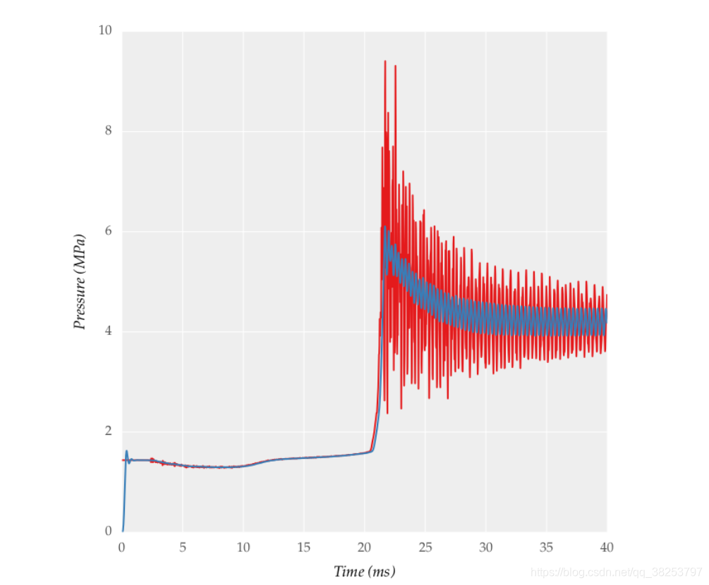
��ɫ������ʵֵ�dz����������������ѿ��������ǾͶ�������һ��ƽ��������ȡ����һ������ֵ��
butter_lowpass_filtfilt�������룺
def butter_lowpass_filtfilt(data, cutoff=1500, fs=50000, order=5):"""��dataֵ����̫��, ��ȡdata��ƽ������"""from scipy.signal import butter, filtfilt# https://stackoverflow.com/questions/28536191/how-to-filter-smooth-with-scipy-numpydef butter_lowpass(cutoff, fs, order):nyq = 0.5 * fsnormal_cutoff = cutoff / nyqreturn butter(order, normal_cutoff, btype='low', analog=False)b, a = butter_lowpass(cutoff, fs, order=order)return filtfilt(b, a, data) # forward-backward filter
\qquad�ⲿ�ֵĴ�������������plot_results_overlay��������ģ���������ע�͵��ģ���������Լ�ѵ���Ľ��������������ֶ����������ҿ��Դ�ע�ͣ��������������������ﵽһ��ƽ��Ч�������������������ÿ�п��ģ�����Ȥ�����Լ��������ͼ���Ӧ�ò��ѡ�
10��feature_visualization
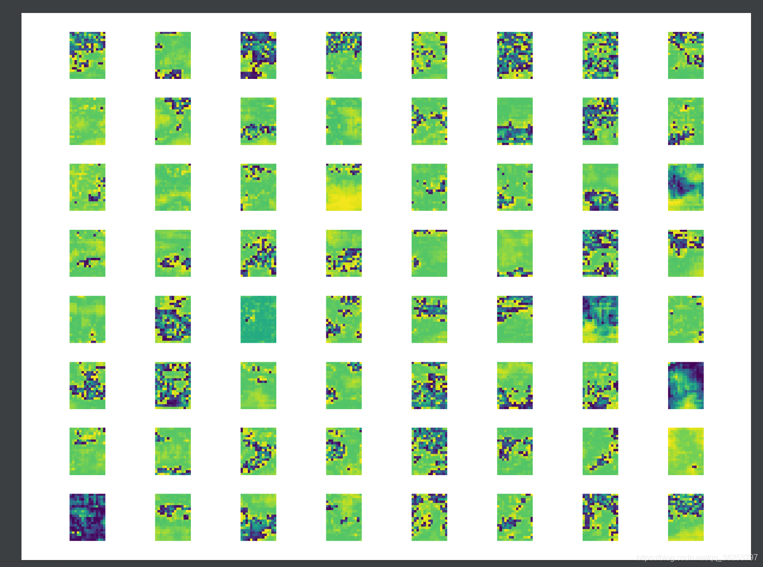
\qquad����������������ӻ�feature map�ģ����ҿ���ʵ�ֿ��ӻ�����������һ���feature map��
�������룺
def feature_visualization(x, module_type, stage, n=64):"""����yolo.py��Model���е�forward_once������ ����ѡ���������п��ӻ��ò�feature map���ӻ�feature map(ģ������㶼������):params x: Features map [bs, channels, height, width]:params module_type: Module type:params stage: Module stage within model:params n: Maximum number of feature maps to plot"""batch, channels, height, width = x.shape # batch, channels, height, widthif height > 1 and width > 1:project, name = 'runs/features', 'exp'save_dir = increment_path(Path(project) / name) # increment runsave_dir.mkdir(parents=True, exist_ok=True) # make save dirplt.figure(tight_layout=True)# torch.chunk: ��torch.cat()ԭ���෴ ��tensor x��dim���л��У��ָ��channels��tensor��, ���ص���һ��Ԫ��# ����2��ά��(channels)��x�ֳ�channels�� ÿ��ͼ������block batch��ͼ blocks=len(blocks)=3*batchblocks = torch.chunk(x, channels, dim=1)n = min(n, len(blocks)) # �ܹ����ӻ���feature map����for i in range(n):feature = transforms.ToPILImage()(blocks[i].squeeze()) # tensor -> PIL Imageax = plt.subplot(int(math.sqrt(n)), int(math.sqrt(n)), i + 1) # ����n�и���n�� ��ǰ���ڵ�i+1����ͼax.axis('off')plt.imshow(feature) # cmap='gray' ���ӻ���ǰfeature mapf = f"stage_{
stage}_{
module_type.split('.')[-1]}_features.png"print(f'Saving {
save_dir / f}...')plt.savefig(save_dir / f, dpi=300)
ͨ����������ǰ�������yolo.py��Model���е�forward_once�����У�
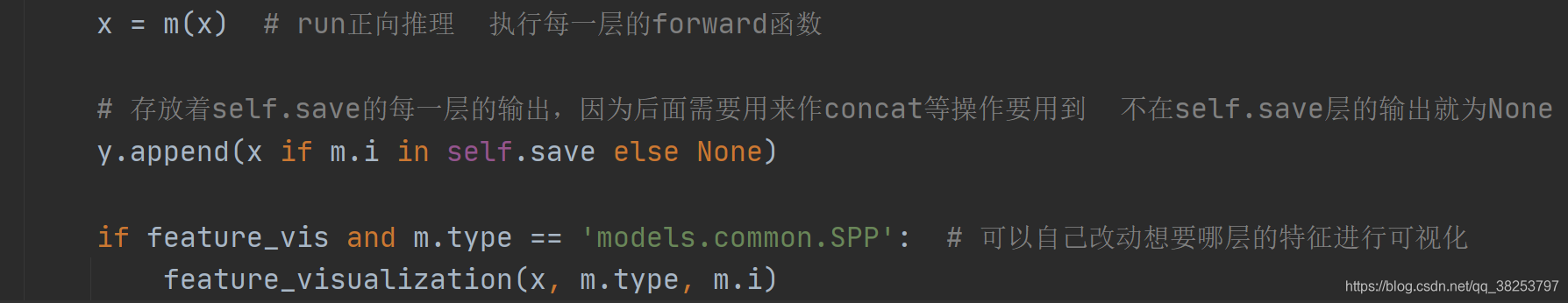
�Լ�������if��ѡ��Ҫ�鿴������һ��feature map��
ԭͼ��
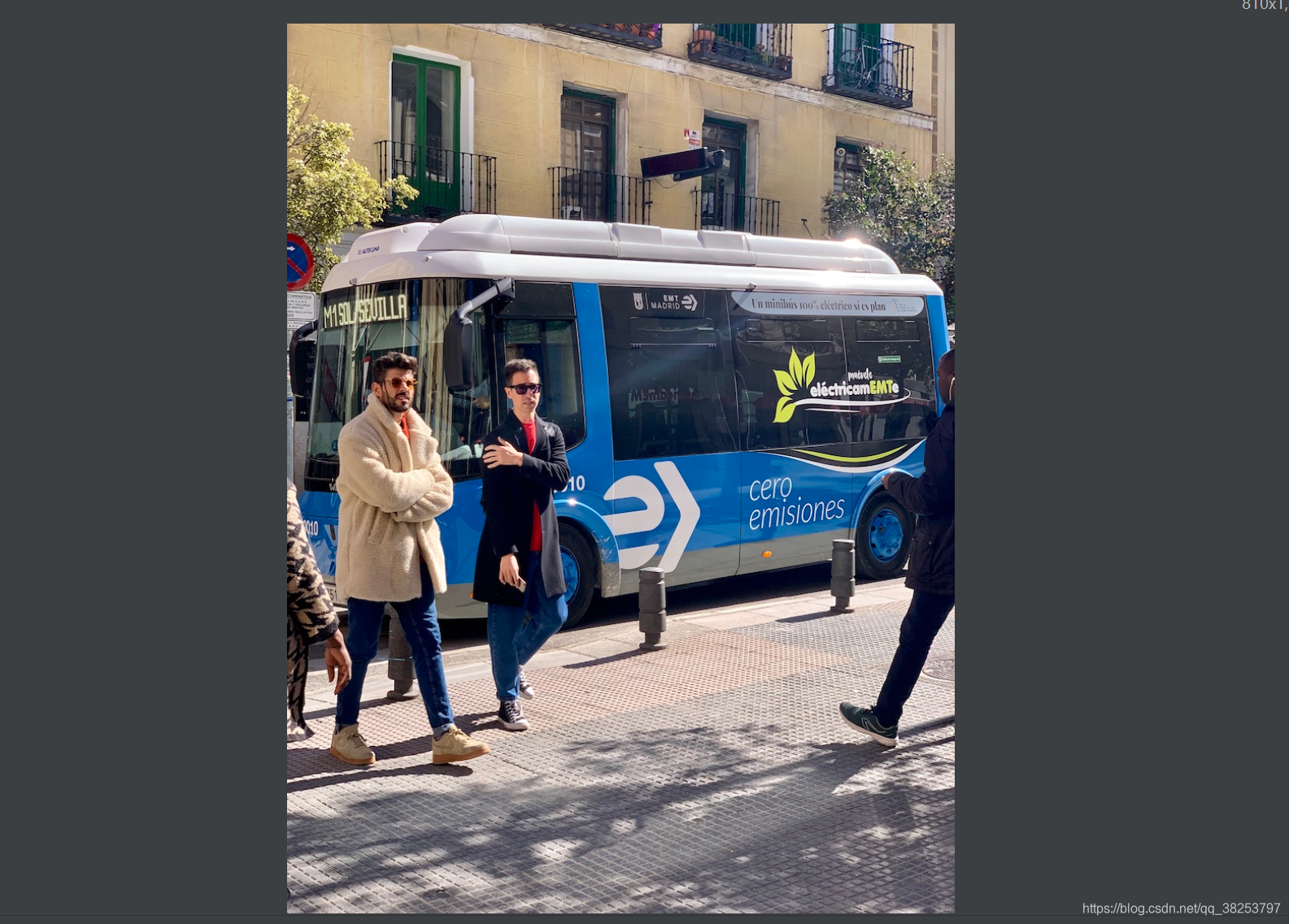
ִ��Ч����
11��plot_study_txt��û�õ�����profile_idetection��û�õ���
\qquadʣ�µ�������������ûʲô�õģ�plot_study_txt��test.py��opt.task == 'study��ʱ����yolov5ϵ�к�yolov3-spp����ģ���ڸ����߶��µ�ָ�겢���ӻ���������ʵ���Ǽ����ò����������һ������profile_idetection��ȫû�õ���������������������Ҳ���ԡ�
def plot_study_txt(path='', x=None):"""û�õ�Plot study.txt generated by test.py"""plot2 = False # plot additional resultsif plot2:ax = plt.subplots(2, 4, figsize=(10, 6), tight_layout=True)[1].ravel()fig2, ax2 = plt.subplots(1, 1, figsize=(8, 4), tight_layout=True)# for f in [Path(path) / f'study_coco_{x}.txt' for x in ['yolov5s6', 'yolov5m6', 'yolov5l6', 'yolov5x6']]:for f in sorted(Path(path).glob('study*.txt')):y = np.loadtxt(f, dtype=np.float32, usecols=[0, 1, 2, 3, 7, 8, 9], ndmin=2).Tx = np.arange(y.shape[1]) if x is None else np.array(x)if plot2:s = ['P', 'R', 'mAP@.5', 'mAP@.5:.95', 't_preprocess (ms/img)', 't_inference (ms/img)', 't_NMS (ms/img)']for i in range(7):ax[i].plot(x, y[i], '.-', linewidth=2, markersize=8)ax[i].set_title(s[i])j = y[3].argmax() + 1ax2.plot(y[5, 1:j], y[3, 1:j] * 1E2, '.-', linewidth=2, markersize=8,label=f.stem.replace('study_coco_', '').replace('yolo', 'YOLO'))ax2.plot(1E3 / np.array([209, 140, 97, 58, 35, 18]), [34.6, 40.5, 43.0, 47.5, 49.7, 51.5],'k.-', linewidth=2, markersize=8, alpha=.25, label='EfficientDet')ax2.grid(alpha=0.2)ax2.set_yticks(np.arange(20, 60, 5))ax2.set_xlim(0, 57)ax2.set_ylim(30, 55)ax2.set_xlabel('GPU Speed (ms/img)')ax2.set_ylabel('COCO AP val')ax2.legend(loc='lower right')plt.savefig(str(Path(path).name) + '.png', dpi=300)def profile_idetection(start=0, stop=0, labels=(), save_dir=''):"""û�õ�Plot iDetection '*.txt' per-image logs"""ax = plt.subplots(2, 4, figsize=(12, 6), tight_layout=True)[1].ravel()s = ['Images', 'Free Storage (GB)', 'RAM Usage (GB)', 'Battery', 'dt_raw (ms)', 'dt_smooth (ms)', 'real-world FPS']files = list(Path(save_dir).glob('frames*.txt'))for fi, f in enumerate(files):try:results = np.loadtxt(f, ndmin=2).T[:, 90:-30] # clip first and last rowsn = results.shape[1] # number of rowsx = np.arange(start, min(stop, n) if stop else n)results = results[:, x]t = (results[0] - results[0].min()) # set t0=0sresults[0] = xfor i, a in enumerate(ax):if i < len(results):label = labels[fi] if len(labels) else f.stem.replace('frames_', '')a.plot(t, results[i], marker='.', label=label, linewidth=1, markersize=5)a.set_title(s[i])a.set_xlabel('time (s)')# if fi == len(files) - 1:# a.set_ylim(bottom=0)for side in ['top', 'right']:a.spines[side].set_visible(False)else:a.remove()except Exception as e:print('Warning: Plotting error for %s; %s' % (f, e))ax[1].legend()plt.savefig(Path(save_dir) / 'idetection_profile.png', dpi=200)
�ܽ�
\qquad����ļ��Ĵ�����Ҫ��һЩ��ͼ�õĹ��ߺ�����������Ŀ�������Ҫ������ʵû��ʲô��ϵ���Ƚ���Ҫ�ĺ����У�plot_one_box��output_to_target��plot_images��plot_labels��plot_evolution��plot_results��plot_results_overlay��feature_visualization�ȡ�
�C2021.08.02 22:14