吴恩达2017深度学习作业-c1w3-Planar data classification with one hidden layer

一、前言

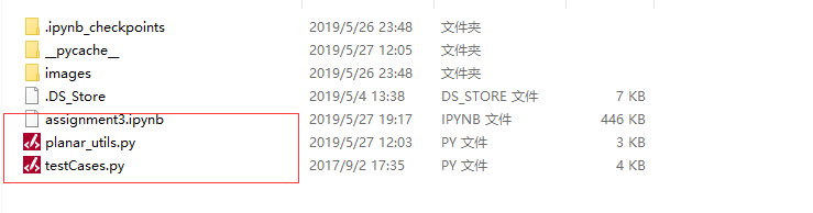
可以去github下载，目录如下，主要是标记的三个文件就可以完成作业。第一个ipynb就是下面次序来的，按照一步一步进行即可，但是要先下载后面两个py文件，在本文后面附上了，下载好后你就可以运行作业，看作业效果啦。

我觉得很巧妙的地方：

1预测时：

.

 

但也有人用了——————  predictions = np.round(A2)  超级赞呢！

 2、梯度的计算

 

搞明白 在numpy中 * 和 np.dot 和np.multiply   三者的区别！我经常搞糊涂。

3、交叉熵损失，为何又是逻辑回归的损失函数？

• 什么时候用softmax？

softmax是一种归一化函数，用于将向量中元素的值都归一化0～1之间，并保持其加和为1。 
公示表达为：

                                                           

                             

根据公式和图片可看出，前一层的激活值越大，经过softmax函数后的值也就越大，又因为softmax的所有输出加和为1，因此，常利用softmax层将激活值与概率实现映射。

举例：

多元分类（multi-class classification）中，每个样本只属于一个类别。将最后一个全连接层输入softmax层，即可得到样本属于每个类别的概率P(yi|X)，注意，这些概率加和等于1

• 什么时候用逻辑回归？

sigmoid函数定义如下：

它表示样本x属于分类Y的概率。

                                                 

由图可以看出，当激活值z很大很大时，P(Y=1|x)接近1，当激活值z很小很小时，P(Y=1|x)接近0.

举例：

多标签分类(multi-label classification )，每个样本可以属于多个类别。将最后一个全连接层输入sigmoid激活函数，最终的每个输出都代表样本属于这个类别的概率即P(Y=1|X)，这些概率加和不等于1.
 

• 那么交叉熵是什么时候使用呢？

用于代价函数。交叉熵H(p,q)用于衡量预测分布q与真实分布p之间的相似度，交叉熵越大，相似度越小。因此，要想让预测的标签的分布与真实的标签分布最接近，就最小化交叉熵啦。 

                                          

举例：

对于二分类问题：(y可取值0或1) 
y_train与y_output的分布的交叉熵表示为：

                        

当y_train为1/0时，y_output也为1/0时交叉熵最小 
Tensorflow中将最后一层全连接层的输出结果 通过使用tf.nn.softmax_cross_entropy_with_logits计算代价函数

对于多标签分类问题(multi-label)和多元分类问题(multi-class) 
交叉熵均可表示为：

                                         

当train_prob的分布与out_prob的分布相同时，交叉熵最小。 
不同点在于： 

对于多标签分类问题： 
Tensorflow中将最后一层全连接层的输出结果 通过使用tf.nn.sigmoid_cross_entropy_with_logits计算代价函数 

对于多元分类问题： 
Tensorflow中将最后一层全连接层的输出结果 通过使用tf.nn.softmax_cross_entropy_with_logits计算代价函数

总结：从上面来看，是根据分类问题的划分去定义使用softmax的交叉熵还sigmoid的交叉熵，其实刚刚

也是交叉熵，只是二分类的交叉熵，那么对于多标签分类问题(multi-label)和多元分类问题(multi-class) 的交叉熵呢？

就是。不要再傻傻分不清逻辑回归，softmax，交叉熵损失等啦

二、正题：

Welcome to your week 3 programming assignment. It's time to build your first neural network, which will have a hidden layer. You will see a big difference between this model and the one you implemented using logistic regression.

You will learn how to:

• Implement a 2-class classification neural network with a single hidden layer
• Use units with a non-linear activation function, such as tanh
• Compute the cross entropy loss
• Implement forward and backward propagation

1 - Packages

Let's first import all the packages that you will need during this assignment.

# Package imports
import numpy as np
import matplotlib.pyplot as plt
from testCases import *
import sklearn
import sklearn.datasets
import sklearn.linear_model
from planar_utils import plot_decision_boundary, sigmoid, load_planar_dataset, load_extra_datasets
from functools import reduce
import operator%matplotlib inlinenp.random.seed(1) # set a seed so that the results are consistent

 

2 - Dataset

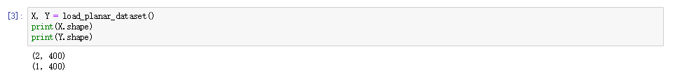
First, let's get the dataset you will work on. The following code will load a "flower" 2-class dataset into variables X and Y.

 

 

 

 Visualize the dataset using matplotlib. The data looks like a "flower" with some red (label y=0) and some blue (y=1) points. Your goal is to build a model to fit this data.

 

You have:

- a numpy-array (matrix) X that contains your features (x1, x2)
- a numpy-array (vector) Y that contains your labels (red:0, blue:1).

Lets first get a better sense of what our data is like.

Exercise: How many training examples do you have? In addition, what is the shape of the variables X and Y?

Hint: How do you get the shape of a numpy array? (help)

### START CODE HERE ### (≈ 3 lines of code)
shape_X = X.shape
shape_Y = Y.shape
m = X.shape[1]  # training set size
### END CODE HERE ###print ('The shape of X is: ' + str(shape_X))
print ('The shape of Y is: ' + str(shape_Y))
print ('I have m = %d training examples!' % (m))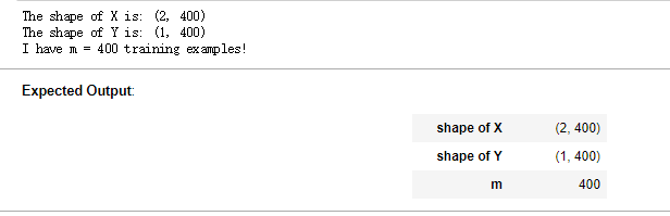

 \

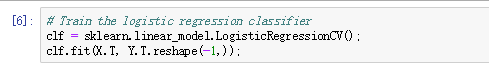
3 - Simple Logistic Regression

Before building a full neural network, lets first see how logistic regression performs on this problem. You can use sklearn's built-in functions to do that. Run the code below to train a logistic regression classifier on the dataset.

You can now plot the decision boundary of these models. Run the code below.

 

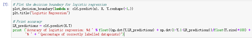
Interpretation: The dataset is not linearly separable, so logistic regression doesn't perform well. Hopefully a neural network will do better. Let's try this now!

4 - Neural Network model

Logistic regression did not work well on the "flower dataset". You are going to train a Neural Network with a single hidden layer.

Here is our model:

转存失败重新上传取消

 

Reminder: The general methodology to build a Neural Network is to:

1. Define the neural network structure ( # of input units,  # of hidden units, etc). 
2. Initialize the model's parameters
3. Loop:- Implement forward propagation- Compute loss- Implement backward propagation to get the gradients- Update parameters (gradient descent)

You often build helper functions to compute steps 1-3 and then merge them into one function we call nn_model(). Once you've built nn_model() and learnt the right parameters, you can make predictions on new data.

4.1 - Defining the neural network structure

Exercise: Define three variables:

- n_x: the size of the input layer
- n_h: the size of the hidden layer (set this to 4) 
- n_y: the size of the output layer

Hint: Use shapes of X and Y to find n_x and n_y. Also, hard code the hidden layer size to be 4.

# GRADED FUNCTION: layer_sizesdef layer_sizes(X, Y):"""Arguments:X -- input dataset of shape (input size, number of examples)Y -- labels of shape (output size, number of examples)Returns:n_x -- the size of the input layern_h -- the size of the hidden layern_y -- the size of the output layer"""### START CODE HERE ### (≈ 3 lines of code)n_x = X.shape[0] # size of input layern_h = 4n_y = Y.shape[0] # size of output layer### END CODE HERE ###return (n_x, n_h, n_y)

4.2 - Initialize the model's parameters

Exercise: Implement the function initialize_parameters().

Instructions:

• Make sure your parameters' sizes are right. Refer to the neural network figure above if needed.
• You will initialize the weights matrices with random values.
  • Use: np.random.randn(a,b) * 0.01 to randomly initialize a matrix of shape (a,b).
• You will initialize the bias vectors as zeros.
  • Use: np.zeros((a,b)) to initialize a matrix of shape (a,b) with zeros.

# GRADED FUNCTION: initialize_parametersdef initialize_parameters(n_x, n_h, n_y):"""Argument:n_x -- size of the input layern_h -- size of the hidden layern_y -- size of the output layerReturns:params -- python dictionary containing your parameters:W1 -- weight matrix of shape (n_h, n_x)b1 -- bias vector of shape (n_h, 1)W2 -- weight matrix of shape (n_y, n_h)b2 -- bias vector of shape (n_y, 1)"""np.random.seed(2) # we set up a seed so that your output matches ours although the initialization is random. 我们设置了一个种子，以便您的输出与我们的匹配，尽管初始化是随机的。### START CODE HERE ### (≈ 4 lines of code)W1 = np.random.randn(n_h,n_x) * 0.01b1 = np.zeros((n_h, 1))W2 = np.random.randn(n_y,n_h) * 0.01b2 = np.zeros((n_y, 1))### END CODE HERE ###assert (W1.shape == (n_h, n_x))assert (b1.shape == (n_h, 1))assert (W2.shape == (n_y, n_h))assert (b2.shape == (n_y, 1))parameters = {"W1": W1,"b1": b1,"W2": W2,"b2": b2}return parameters

4.3 - The Loop

Question: Implement forward_propagation().

# GRADED FUNCTION: forward_propagationdef forward_propagation(X, parameters):"""Argument:X -- input data of size (n_x, m)parameters -- python dictionary containing your parameters (output of initialization function)Returns:A2 -- The sigmoid output of the second activationcache -- a dictionary containing "Z1", "A1", "Z2" and "A2""""# Retrieve each parameter from the dictionary "parameters"### START CODE HERE ### (≈ 4 lines of code)W1 = parameters["W1"]b1 = parameters["b1"]W2 = parameters["W2"]b2 = parameters["b2"]### END CODE HERE #### Implement Forward Propagation to calculate A2 (probabilities)### START CODE HERE ### (≈ 4 lines of code)Z1 = np.dot(W1,X)+b1A1 = np.tanh(Z1)Z2 = np.dot(W2,A1)+b2A2 = sigmoid(Z2)### END CODE HERE ###assert(A2.shape == (1, X.shape[1]))cache = {"Z1": Z1,"A1": A1,"Z2": Z2,"A2": A2}return A2, cache

 

# GRADED FUNCTION: compute_costdef compute_cost(A2, Y, parameters):"""Computes the cross-entropy cost given in equation (13)Arguments:A2 -- The sigmoid output of the second activation, of shape (1, number of examples)Y -- "true" labels vector of shape (1, number of examples)parameters -- python dictionary containing your parameters W1, b1, W2 and b2Returns:cost -- cross-entropy cost given equation (13)"""m = Y.shape[1] # number of example# Compute the cross-entropy cost### START CODE HERE ### (≈ 2 lines of code)#logprobs = np.multiply(np.log(A2), Y)#cost = - np.sum(logprobs)logprobs = np.multiply(np.log(A2), Y) + np.multiply(np.log(1-A2), 1-Y)cost = - 1/m * np.sum(logprobs)### END CODE HERE ###cost = np.squeeze(cost)     # makes sure cost is the dimension we expect. # E.g., turns [[17]] into 17 assert(isinstance(cost, float))return cost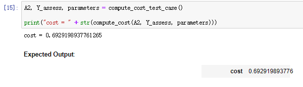

Using the cache computed during forward propagation, you can now implement backward propagation.

Question: Implement the function backward_propagation().

Instructions: Backpropagation is usually the hardest (most mathematical) part in deep learning. To help you, here again is the slide from the lecture on backpropagation. You'll want to use the six equations on the right of this slide, since you are building a vectorized implementation.

# GRADED FUNCTION: backward_propagationdef backward_propagation(parameters, cache, X, Y):"""Implement the backward propagation using the instructions above.Arguments:parameters -- python dictionary containing our parameters cache -- a dictionary containing "Z1", "A1", "Z2" and "A2".X -- input data of shape (2, number of examples)Y -- "true" labels vector of shape (1, number of examples)Returns:grads -- python dictionary containing your gradients with respect to different parameters"""m = X.shape[1]# First, retrieve W1 and W2 from the dictionary "parameters".### START CODE HERE ### (≈ 2 lines of code)W1 = parameters["W1"]W2 = parameters["W2"]### END CODE HERE #### Retrieve also A1 and A2 from dictionary "cache".### START CODE HERE ### (≈ 2 lines of code)A1 = cache["A1"]A2 = cache["A2"]### END CODE HERE #### Backward propagation: calculate dW1, db1, dW2, db2. ### START CODE HERE ### (≈ 6 lines of code, corresponding to 6 equations on slide above)dZ2 = A2 -YdW2 = 1/m * np.dot(dZ2, A1.T)db2 = 1/m * np.sum(dZ2, axis=1, keepdims=True)dZ1 = np.multiply(np.dot(W2.T, dZ2),1-np.power(A1, 2))dW1 = 1/m * np.dot(dZ1, X.T)db1 = 1/m * np.sum(dZ1, axis=1, keepdims=True)### END CODE HERE ###grads = {"dW1": dW1,"db1": db1,"dW2": dW2,"db2": db2}return grads

                                                                      

# GRADED FUNCTION: update_parametersdef update_parameters(parameters, grads, learning_rate = 1.2):"""Updates parameters using the gradient descent update rule given aboveArguments:parameters -- python dictionary containing your parameters grads -- python dictionary containing your gradients Returns:parameters -- python dictionary containing your updated parameters """# Retrieve each parameter from the dictionary "parameters"### START CODE HERE ### (≈ 4 lines of code)W1 = parameters["W1"]b1 = parameters["b1"]W2 = parameters["W2"]b2 = parameters["b2"]### END CODE HERE #### Retrieve each gradient from the dictionary "grads"### START CODE HERE ### (≈ 4 lines of code)dW1 = grads["dW1"]db1 = grads["db1"]dW2 = grads["dW2"]db2 = grads["db2"]## END CODE HERE #### Update rule for each parameter### START CODE HERE ### (≈ 4 lines of code)W1 -= learning_rate * dW1b1 -= learning_rate * db1W2 -= learning_rate * dW2b2 -= learning_rate * db2### END CODE HERE ###parameters = {"W1": W1,"b1": b1,"W2": W2,"b2": b2}return parameters

 

4.4 - Integrate parts 4.1, 4.2 and 4.3 in nn_model()

Question: Build your neural network model in nn_model().

Instructions: The neural network model has to use the previous functions in the right order.

# GRADED FUNCTION: nn_modeldef nn_model(X, Y, n_h, num_iterations = 10000, print_cost=False):"""Arguments:X -- dataset of shape (2, number of examples)Y -- labels of shape (1, number of examples)n_h -- size of the hidden layernum_iterations -- Number of iterations in gradient descent loopprint_cost -- if True, print the cost every 1000 iterationsReturns:parameters -- parameters learnt by the model. They can then be used to predict."""np.random.seed(3)n_x = layer_sizes(X, Y)[0]n_y = layer_sizes(X, Y)[2]# Initialize parameters, then retrieve W1, b1, W2, b2. Inputs: "n_x, n_h, n_y". Outputs = "W1, b1, W2, b2, parameters".### START CODE HERE ### (≈ 5 lines of code)parameters = initialize_parameters(n_x, n_h, n_y)W1 = parameters["W1"]b1 = parameters["b1"]W2 = parameters["W2"]b2 = parameters["b2"]### END CODE HERE #### Loop (gradient descent)for i in range(0, num_iterations):### START CODE HERE ### (≈ 4 lines of code)# Forward propagation. Inputs: "X, parameters". Outputs: "A2, cache".A2, cache = forward_propagation(X, parameters)# Cost function. Inputs: "A2, Y, parameters". Outputs: "cost".cost = compute_cost(A2, Y, parameters)# Backpropagation. Inputs: "parameters, cache, X, Y". Outputs: "grads".grads = backward_propagation(parameters, cache, X, Y)# Gradient descent parameter update. Inputs: "parameters, grads". Outputs: "parameters".parameters = update_parameters(parameters, grads)### END CODE HERE #### Print the cost every 1000 iterationsif print_cost and i % 1000 == 0:print ("Cost after iteration %i: %f" %(i, cost))return parameters

4.5 Predictions

Question: Use your model to predict by building predict(). Use forward propagation to predict results.

# GRADED FUNCTION: predictdef predict(parameters, X):"""Using the learned parameters, predicts a class for each example in XArguments:parameters -- python dictionary containing your parameters X -- input data of size (n_x, m)Returnspredictions -- vector of predictions of our model (red: 0 / blue: 1)"""# Computes probabilities using forward propagation, and classifies to 0/1 using 0.5 as the threshold.### START CODE HERE ### (≈ 2 lines of code)A2, cache = forward_propagation(X, parameters)#print(A2)predictions =  (A2>0.5)### END CODE HERE ###return predictions

 

 

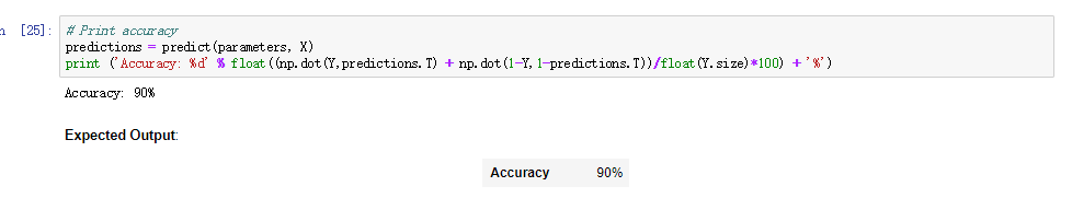
Accuracy is really high compared to Logistic Regression. The model has learnt the leaf patterns of the flower! Neural networks are able to learn even highly non-linear decision boundaries, unlike logistic regression.

Now, let's try out several hidden layer sizes.

4.6 - Tuning hidden layer size (optional/ungraded exercise)

Run the following code. It may take 1-2 minutes. You will observe different behaviors of the model for various hidden layer sizes.

Interpretation:

• The larger models (with more hidden units) are able to fit the training set better, until eventually the largest models overfit the data.
• The best hidden layer size seems to be around n_h = 5. Indeed, a value around here seems to fits the data well without also incurring noticable overfitting.
• You will also learn later about regularization, which lets you use very large models (such as n_h = 50) without much overfitting.

Optional questions:

Note: Remember to submit the assignment but clicking the blue "Submit Assignment" button at the upper-right.

Some optional/ungraded questions that you can explore if you wish:

• What happens when you change the tanh activation for a sigmoid activation or a ReLU activation?
• Play with the learning_rate. What happens?
• What if we change the dataset? (See part 5 below!)

 

You've learnt to:

• Build a complete neural network with a hidden layer
• Make a good use of a non-linear unit
• Implemented forward propagation and backpropagation, and trained a neural network
• See the impact of varying the hidden layer size, including overfitting.

 

Nice work!

 

5) Performance on other datasets

If you want, you can rerun the whole notebook (minus the dataset part) for each of the following datasets.

你可以改变上面的数据，进行不同的分类~看看你的网络的怎么强大法~ 

# This may take about 2 minutes to runplt.figure(figsize=(16, 32))
hidden_layer_sizes = [1, 2, 3, 4, 5, 10, 20]
for i, n_h in enumerate(hidden_layer_sizes):plt.subplot(5, 2, i+1)plt.title('Hidden Layer of size %d' % n_h)parameters = nn_model(X, Y, n_h, num_iterations = 5000)plot_decision_boundary(lambda x: predict(parameters, x.T), X, Y.reshape(-1,))predictions = predict(parameters, X)accuracy = float((np.dot(Y,predictions.T) + np.dot(1-Y,1-predictions.T))/float(Y.size)*100)print ("Accuracy for {} hidden units: {} %".format(n_h, accuracy))

Reference:

• http://scs.ryerson.ca/~aharley/neural-networks/
• http://cs231n.github.io/neural-networks-case-study/

 planar_utils.py

import matplotlib.pyplot as plt
import numpy as np
import sklearn
import sklearn.datasets
import sklearn.linear_modeldef plot_decision_boundary(model, X, y):# Set min and max values and give it some paddingx_min, x_max = X[0, :].min() - 1, X[0, :].max() + 1y_min, y_max = X[1, :].min() - 1, X[1, :].max() + 1h = 0.01# Generate a grid of points with distance h between themxx, yy = np.meshgrid(np.arange(x_min, x_max, h), np.arange(y_min, y_max, h))# Predict the function value for the whole gridZ = model(np.c_[xx.ravel(), yy.ravel()])Z = Z.reshape(xx.shape)# Plot the contour and training examplesplt.contourf(xx, yy, Z, cmap=plt.cm.Spectral)plt.ylabel('x2')plt.xlabel('x1')plt.scatter(X[0, :], X[1, :], c=y, cmap=plt.cm.Spectral)def sigmoid(x):"""Compute the sigmoid of xArguments:x -- A scalar or numpy array of any size.Return:s -- sigmoid(x)"""#x.astype(np.float64)s = 1/(1+np.exp(-x))return sdef load_planar_dataset():np.random.seed(1)m = 400 # number of examplesN = int(m/2) # number of points per classD = 2 # dimensionalityX = np.zeros((m,D)) # data matrix where each row is a single exampleY = np.zeros((m,1), dtype='uint8') # labels vector (0 for red, 1 for blue)a = 4 # maximum ray of the flowerfor j in range(2):ix = range(N*j,N*(j+1))t = np.linspace(j*3.12,(j+1)*3.12,N) + np.random.randn(N)*0.2 # thetar = a*np.sin(4*t) + np.random.randn(N)*0.2 # radiusX[ix] = np.c_[r*np.sin(t), r*np.cos(t)]Y[ix] = jX = X.TY = Y.Treturn X, Ydef load_extra_datasets():  N = 200noisy_circles = sklearn.datasets.make_circles(n_samples=N, factor=.5, noise=.3)noisy_moons = sklearn.datasets.make_moons(n_samples=N, noise=.2)blobs = sklearn.datasets.make_blobs(n_samples=N, random_state=5, n_features=2, centers=6)gaussian_quantiles = sklearn.datasets.make_gaussian_quantiles(mean=None, cov=0.5, n_samples=N, n_features=2, n_classes=2, shuffle=True, random_state=None)no_structure = np.random.rand(N, 2), np.random.rand(N, 2)return noisy_circles, noisy_moons, blobs, gaussian_quantiles, no_structure

 testCases.py

 

import numpy as npdef layer_sizes_test_case():np.random.seed(1)X_assess = np.random.randn(5, 3)Y_assess = np.random.randn(2, 3)return X_assess, Y_assessdef initialize_parameters_test_case():n_x, n_h, n_y = 2, 4, 1return n_x, n_h, n_ydef forward_propagation_test_case():np.random.seed(1)X_assess = np.random.randn(2, 3)parameters = {'W1': np.array([[-0.00416758, -0.00056267],[-0.02136196,  0.01640271],[-0.01793436, -0.00841747],[ 0.00502881, -0.01245288]]),'W2': np.array([[-0.01057952, -0.00909008,  0.00551454,  0.02292208]]),'b1': np.array([[ 0.],[ 0.],[ 0.],[ 0.]]),'b2': np.array([[ 0.]])}return X_assess, parametersdef compute_cost_test_case():np.random.seed(1)Y_assess = np.random.randn(1, 3)parameters = {'W1': np.array([[-0.00416758, -0.00056267],[-0.02136196,  0.01640271],[-0.01793436, -0.00841747],[ 0.00502881, -0.01245288]]),'W2': np.array([[-0.01057952, -0.00909008,  0.00551454,  0.02292208]]),'b1': np.array([[ 0.],[ 0.],[ 0.],[ 0.]]),'b2': np.array([[ 0.]])}a2 = (np.array([[ 0.5002307 ,  0.49985831,  0.50023963]]))return a2, Y_assess, parametersdef backward_propagation_test_case():np.random.seed(1)X_assess = np.random.randn(2, 3)Y_assess = np.random.randn(1, 3)parameters = {'W1': np.array([[-0.00416758, -0.00056267],[-0.02136196,  0.01640271],[-0.01793436, -0.00841747],[ 0.00502881, -0.01245288]]),'W2': np.array([[-0.01057952, -0.00909008,  0.00551454,  0.02292208]]),'b1': np.array([[ 0.],[ 0.],[ 0.],[ 0.]]),'b2': np.array([[ 0.]])}cache = {'A1': np.array([[-0.00616578,  0.0020626 ,  0.00349619],[-0.05225116,  0.02725659, -0.02646251],[-0.02009721,  0.0036869 ,  0.02883756],[ 0.02152675, -0.01385234,  0.02599885]]),'A2': np.array([[ 0.5002307 ,  0.49985831,  0.50023963]]),'Z1': np.array([[-0.00616586,  0.0020626 ,  0.0034962 ],[-0.05229879,  0.02726335, -0.02646869],[-0.02009991,  0.00368692,  0.02884556],[ 0.02153007, -0.01385322,  0.02600471]]),'Z2': np.array([[ 0.00092281, -0.00056678,  0.00095853]])}return parameters, cache, X_assess, Y_assessdef update_parameters_test_case():parameters = {'W1': np.array([[-0.00615039,  0.0169021 ],[-0.02311792,  0.03137121],[-0.0169217 , -0.01752545],[ 0.00935436, -0.05018221]]),'W2': np.array([[-0.0104319 , -0.04019007,  0.01607211,  0.04440255]]),'b1': np.array([[ -8.97523455e-07],[  8.15562092e-06],[  6.04810633e-07],[ -2.54560700e-06]]),'b2': np.array([[  9.14954378e-05]])}grads = {'dW1': np.array([[ 0.00023322, -0.00205423],[ 0.00082222, -0.00700776],[-0.00031831,  0.0028636 ],[-0.00092857,  0.00809933]]),'dW2': np.array([[ -1.75740039e-05,   3.70231337e-03,  -1.25683095e-03,-2.55715317e-03]]),'db1': np.array([[  1.05570087e-07],[ -3.81814487e-06],[ -1.90155145e-07],[  5.46467802e-07]]),'db2': np.array([[ -1.08923140e-05]])}return parameters, gradsdef nn_model_test_case():np.random.seed(1)X_assess = np.random.randn(2, 3)Y_assess = np.random.randn(1, 3)return X_assess, Y_assessdef predict_test_case():np.random.seed(1)X_assess = np.random.randn(2, 3)parameters = {'W1': np.array([[-0.00615039,  0.0169021 ],[-0.02311792,  0.03137121],[-0.0169217 , -0.01752545],[ 0.00935436, -0.05018221]]),'W2': np.array([[-0.0104319 , -0.04019007,  0.01607211,  0.04440255]]),'b1': np.array([[ -8.97523455e-07],[  8.15562092e-06],[  6.04810633e-07],[ -2.54560700e-06]]),'b2': np.array([[  9.14954378e-05]])}return parameters, X_assess