吴恩达2017深度学习作业-c2w1-Optimization Methods（下）_综合

这次作业其实总的来说花费了很长时间，主要是自己不能集中去写代码，第二是基础知识很多不扎实，很多需要查，但是我查也不是深究，我就简单记录一下用法，主要还是需要多用。每次都小结一下。

前面一些错误的点：

 s["dW" + str(l+1)] = beta2 * s["dW" + str(l+1)] + (1-beta2)* np.square(grads["dW" + str(l+1)])#s["db" + str(l+1)] = beta2 * s["db" + str(l+1)] + (1-beta2)* math.pow(grads["db" + str(l+1)],2) 错啦

 v_corrected["dW" + str(l+1)] = v["dW" + str(l+1)] / (1 - np.power(beta1,t))
#v_corrected["db" + str(l+1)] = v["db" + str(l+1)] / (1 - math.pow(beta1,l)) 错啦

新的写法：

  s["dW"+str(l+1)]=np.zeros((parameters["W"+str(l+1)].shape[0],parameters["W"+str(l+1)].shape[1]))s["db" + str(l+1)] = np.zeros_like(parameters['b'+ str(l+1)])

新学的函数：

numpy中的ravel()、flatten()、squeeze()的用法与区别 https://blog.csdn.net/tymatlab/article/details/79009618

参见官方文档：

ravel()
flatten()
squeeze()

Python Numpy模块函数np.c_和np.r_学习使用 https://blog.csdn.net/Together_CZ/article/details/79548217

np.r_是按行连接两个矩阵，就是把两矩阵上下相加，要求行数相等，类似于pandas中的concat()
np.c_是按列连接两个矩阵，就是把两矩阵左右相加，要求列数相等，类似于pandas中的merge()

5 - Model with different optimization algorithms

Lets use the following "moons" dataset to test the different optimization methods. (The dataset is named "moons" because the data from each of the two classes looks a bit like a crescent-shaped moon.)

train_X, train_Y = load_dataset()print(train_X.shape[0],train_X.shape[1])
print(train_X[:,0])
print(train_X[0,:])
print(train_Y.shape[0],train_Y.shape[1])
print(train_Y)
print(train_Y.flatten())

We have already implemented a 3-layer neural network. You will train it with:

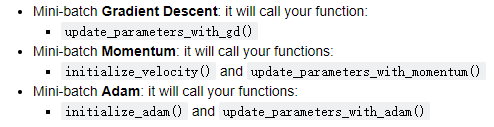
def model(X, Y, layers_dims, optimizer, learning_rate = 0.0007, mini_batch_size = 64, beta = 0.9,beta1 = 0.9, beta2 = 0.999,  epsilon = 1e-8, num_epochs = 10000, print_cost = True):"""3-layer neural network model which can be run in different optimizer modes.Arguments:X -- input data, of shape (2, number of examples)Y -- true "label" vector (1 for blue dot / 0 for red dot), of shape (1, number of examples)layers_dims -- python list, containing the size of each layerlearning_rate -- the learning rate, scalar.mini_batch_size -- the size of a mini batchbeta -- Momentum hyperparameterbeta1 -- Exponential decay hyperparameter for the past gradients estimates beta2 -- Exponential decay hyperparameter for the past squared gradients estimates epsilon -- hyperparameter preventing division by zero in Adam updatesnum_epochs -- number of epochsprint_cost -- True to print the cost every 1000 epochsReturns:parameters -- python dictionary containing your updated parameters """L = len(layers_dims)             # number of layers in the neural networkscosts = []                       # to keep track of the costt = 0                            # initializing the counter required for Adam update 初始化Adam更新所需的计数器seed = 10                        # For grading purposes, so that your "random" minibatches are the same as ours# Initialize parametersparameters = initialize_parameters(layers_dims)# Initialize the optimizerif optimizer == "gd":pass # no initialization required for gradient descentelif optimizer == "momentum":v = initialize_velocity(parameters)elif optimizer == "adam":v, s = initialize_adam(parameters)# Optimization loopfor i in range(num_epochs):# Define the random minibatches. We increment the seed to reshuffle differently the dataset after each epoch#定义随机的小批。我们增加种子以在每个历元之后以不同的方式重新洗牌数据集seed = seed + 1minibatches = random_mini_batches(X, Y, mini_batch_size, seed)for minibatch in minibatches:# Select a minibatch(minibatch_X, minibatch_Y) = minibatch# Forward propagationa3, caches = forward_propagation(minibatch_X, parameters)# Compute costcost = compute_cost(a3, minibatch_Y)# Backward propagationgrads = backward_propagation(minibatch_X, minibatch_Y, caches)# Update parametersif optimizer == "gd":parameters = update_parameters_with_gd(parameters, grads, learning_rate) #梯度下降算法（小批量）elif optimizer == "momentum":parameters, v = update_parameters_with_momentum(parameters, grads, v, beta, learning_rate)elif optimizer == "adam":t = t + 1 # Adam counterparameters, v, s = update_parameters_with_adam(parameters, grads, v, s,t, learning_rate, beta1, beta2,  epsilon)# Print the cost every 1000 epochif print_cost and i % 1000 == 0:print ("Cost after epoch %i: %f" %(i, cost))if print_cost and i % 100 == 0:costs.append(cost)# plot the costplt.plot(costs)plt.ylabel('cost')plt.xlabel('epochs (per 100)')plt.title("Learning rate = " + str(learning_rate))plt.show()return parameters

You will now run this 3 layer neural network with each of the 3 optimization methods.

5.1 - Mini-batch Gradient descent

Run the following code to see how the model does with mini-batch gradient descent.

# train 3-layer model
layers_dims = [train_X.shape[0], 5, 2, 1]
parameters = model(train_X, train_Y, layers_dims, optimizer = "gd")# Predict
predictions = predict(train_X, train_Y, parameters)
print(predictions)
# Plot decision boundary
plt.title("Model with Gradient Descent optimization")
axes = plt.gca() #gca=get current axis
axes.set_xlim([-1.5,2.5])
axes.set_ylim([-1,1.5])
# print(x.T)
plot_decision_boundary(lambda x: predict_dec(parameters, x.T), train_X, train_Y.flatten())

5.2 - Mini-batch gradient descent with momentum

Run the following code to see how the model does with momentum. Because this example is relatively simple, the gains from using momemtum are small; but for more complex problems you might see bigger gains.运行以下代码，查看模型如何处理动量。因为这个例子相对简单，使用momemtum的收益很小;但对于更复杂的问题，你可能会看到更大的收益。

# train 3-layer model
layers_dims = [train_X.shape[0], 5, 2, 1]
parameters = model(train_X, train_Y, layers_dims, beta = 0.9, optimizer = "momentum")# Predict
predictions = predict(train_X, train_Y, parameters)# Plot decision boundary
plt.title("Model with Momentum optimization")
axes = plt.gca()
axes.set_xlim([-1.5,2.5])
axes.set_ylim([-1,1.5])
plot_decision_boundary(lambda x: predict_dec(parameters, x.T), train_X, train_Y.flatten())

5.3 - Mini-batch with Adam mode

Run the following code to see how the model does with Adam.

# train 3-layer model
layers_dims = [train_X.shape[0], 5, 2, 1]
parameters = model(train_X, train_Y, layers_dims, optimizer = "adam")# Predict
predictions = predict(train_X, train_Y, parameters)# Plot decision boundary
plt.title("Model with Adam optimization")
axes = plt.gca()
axes.set_xlim([-1.5,2.5])
axes.set_ylim([-1,1.5])
plot_decision_boundary(lambda x: predict_dec(parameters, x.T), train_X, train_Y.flatten())

5.4 - Summary

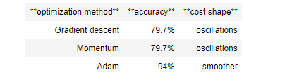
Momentum usually helps, but given the small learning rate and the simplistic dataset, its impact is almost negligeable. Also, the huge oscillations you see in the cost come from the fact that some minibatches are more difficult thans others for the optimization algorithm.

Adam on the other hand, clearly outperforms mini-batch gradient descent and Momentum. If you run the model for more epochs on this simple dataset, all three methods will lead to very good results. However, you've seen that Adam converges a lot faster. 动量通常是有帮助的，但是考虑到较小的学习速度和简单的数据集，它的影响几乎是可以忽略的。此外，您在成本中看到的巨大振荡来自于这样一个事实，即一些小批量比其他优化算法更困难。另一方面，Adam明显优于小批量梯度下降和动量。如果您在这个简单的数据集中运行模型更长的时间，那么这三种方法都将带来非常好的结果。不过，你已经看到Adam收敛得更快了。

Some advantages of Adam include:

Relatively low memory requirements (though higher than gradient descent and gradient descent with momentum)
Usually works well even with little tuning of hyperparameters (except αα) Adam的一些优点包括: 相对较低的内存需求(虽然比梯度下降和带动量的梯度下降要高) 通常，即使很少调整超参数也能很好地工作（除了学习率）

References:

Adam paper: https://arxiv.org/pdf/1412.6980.pdf