文章作者：Tyan
博客：noahsnail.com  |  CSDN  |  简书

声明：作者翻译论文仅为学习，如有侵权请联系作者删除博文，谢谢！

翻译论文汇总：https://github.com/SnailTyan/deep-learning-papers-translation

Going Deeper with Convolutions

Abstract

We propose a deep convolutional neural network architecture codenamed Inception that achieves the new state of the art for classification and detection in the ImageNet Large-Scale Visual Recognition Challenge 2014 (ILSVRC14). The main hallmark of this architecture is the improved utilization of the computing resources inside the network. By a carefully crafted design, we increased the depth and width of the network while keeping the computational budget constant. To optimize quality, the architectural decisions were based on the Hebbian principle and the intuition of multi-scale processing. One particular incarnation used in our submission for ILSVRC14 is called GoogLeNet, a 22 layers deep network, the quality of which is assessed in the context of classification and detection.

我们在ImageNet大规模视觉识别挑战赛2014（ILSVRC14）上提出了一种代号为Inception的深度卷积神经网络结构，并在分类和检测上取得了新的最好结果。这个架构的主要特点是提高了网络内部计算资源的利用率。通过精心的手工设计，我们在增加了网络深度和广度的同时保持了计算预算不变。为了优化质量，架构的设计以赫布理论和多尺度处理直觉为基础。我们在ILSVRC14提交中应用的一个特例被称为GoogLeNet，一个22层的深度网络，其质量在分类和检测的背景下进行了评估。

1. Introduction

In the last three years, our object classification and detection capabilities have dramatically improved due to advances in deep learning and convolutional networks [10]. One encouraging news is that most of this progress is not just the result of more powerful hardware, larger datasets and bigger models, but mainly a consequence of new ideas, algorithms and improved network architectures. No new data sources were used, for example, by the top entries in the ILSVRC 2014 competition besides the classification dataset of the same competition for detection purposes. Our GoogLeNet submission to ILSVRC 2014 actually uses 12 times fewer parameters than the winning architecture of Krizhevsky et al [9] from two years ago, while being significantly more accurate. On the object detection front, the biggest gains have not come from naive application of bigger and bigger deep networks, but from the synergy of deep architectures and classical computer vision, like the R-CNN algorithm by Girshick et al [6].

1. 引言

过去三年中，由于深度学习和卷积网络的发展[10]，我们的目标分类和检测能力得到了显著提高。一个令人鼓舞的消息是，大部分的进步不仅仅是更强大硬件、更大数据集、更大模型的结果，而主要是新的想法、算法和网络结构改进的结果。例如，ILSVRC 2014竞赛中最靠前的输入除了用于检测目的的分类数据集之外，没有使用新的数据资源。我们在ILSVRC 2014中的GoogLeNet提交实际使用的参数只有两年前Krizhevsky等人[9]获胜结构参数的1/12，而结果明显更准确。在目标检测前沿，最大的收获不是来自于越来越大的深度网络的简单应用，而是来自于深度架构和经典计算机视觉的协同，像Girshick等人[6]的R-CNN算法那样。

Another notable factor is that with the ongoing traction of mobile and embedded computing, the efficiency of our algorithms —— especially their power and memory use —— gains importance. It is noteworthy that the considerations leading to the design of the deep architecture presented in this paper included this factor rather than having a sheer fixation on accuracy numbers. For most of the experiments, the models were designed to keep a computational budget of 1.5 billion multiply-adds at inference time, so that the they do not end up to be a purely academic curiosity, but could be put to real world use, even on large datasets, at a reasonable cost.

另一个显著因素是随着移动和嵌入式设备的推动，我们的算法的效率很重要——尤其是它们的电力和内存使用。值得注意的是，正是包含了这个因素的考虑才得出了本文中呈现的深度架构设计，而不是单纯的为了提高准确率。对于大多数实验来说，模型被设计为在一次推断中保持15亿乘加的计算预算，所以最终它们不是单纯的学术好奇心，而是能在现实世界中应用，甚至是以合理的代价在大型数据集上使用。

In this paper, we will focus on an efficient deep neural network architecture for computer vision, codenamed Inception, which derives its name from the Network in network paper by Lin et al [12] in conjunction with the famous “we need to go deeper” internet meme [1]. In our case, the word “deep” is used in two different meanings: first of all, in the sense that we introduce a new level of organization in the form of the “Inception module” and also in the more direct sense of increased network depth. In general, one can view the Inception model as a logical culmination of [12] while taking inspiration and guidance from the theoretical work by Arora et al [2]. The benefits of the architecture are experimentally verified on the ILSVRC 2014 classification and detection challenges, where it significantly outperforms the current state of the art.

在本文中，我们将关注一个高效的计算机视觉深度神经网络架构，代号为Inception，它的名字来自于Lin等人[12]网络论文中的Network与著名的“we need to go deeper”网络迷因[1]的结合。在我们的案例中，单词“deep”用在两个不同的含义中：首先，在某种意义上，我们以“Inception module”的形式引入了一种新层次的组织方式，在更直接的意义上增加了网络的深度。一般来说，可以把Inception模型看作论文[12]的逻辑顶点同时从Arora等人[2]的理论工作中受到了鼓舞和引导。这种架构的好处在ILSVRC 2014分类和检测挑战赛中通过实验得到了验证，它明显优于目前的最好水平。

2. Related Work

Starting with LeNet-5 [10], convolutional neural networks (CNN) have typically had a standard structure —— stacked convolutional layers (optionally followed by contrast normalization and max-pooling) are followed by one or more fully-connected layers. Variants of this basic design are prevalent in the image classification literature and have yielded the best results to-date on MNIST, CIFAR and most notably on the ImageNet classification challenge [9, 21]. For larger datasets such as Imagenet, the recent trend has been to increase the number of layers [12] and layer size [21, 14], while using dropout [7] to address the problem of overfitting.

2. 近期工作

从LeNet-5 [10]开始，卷积神经网络（CNN）通常有一个标准结构——堆叠的卷积层（后面可以选择有对比归一化和最大池化）后面是一个或更多的全连接层。这个基本设计的变种在图像分类著作流行，并且目前为止在MNIST，CIFAR和更著名的ImageNet分类挑战赛中[9, 21]的已经取得了最佳结果。对于更大的数据集例如ImageNet来说，最近的趋势是增加层的数目[12]和层的大小[21, 14]，同时使用丢弃[7]来解决过拟合问题。

Despite concerns that max-pooling layers result in loss of accurate spatial information, the same convolutional network architecture as [9] has also been successfully employed for localization [9, 14], object detection [6, 14, 18, 5] and human pose estimation [19].

尽管担心最大池化层会引起准确空间信息的损失，但与[9]相同的卷积网络结构也已经成功的应用于定位[9, 14]，目标检测[6, 14, 18, 5]和行人姿态估计[19]。

Inspired by a neuroscience model of the primate visual cortex, Serre et al. [15] used a series of fixed Gabor filters of different sizes to handle multiple scales. We use a similar strategy here. However, contrary to the fixed 2-layer deep model of [15], all filters in the Inception architecture are learned. Furthermore, Inception layers are repeated many times, leading to a 22-layer deep model in the case of the GoogLeNet model.

受灵长类视觉皮层神经科学模型的启发，Serre等人[15]使用了一系列固定的不同大小的Gabor滤波器来处理多尺度。我们使用一个了类似的策略。然而，与[15]的固定的2层深度模型相反，Inception结构中所有的滤波器是学习到的。此外，Inception层重复了很多次，在GoogLeNet模型中得到了一个22层的深度模型。

Network-in-Network is an approach proposed by Lin et al. [12] in order to increase the representational power of neural networks. In their model, additional 1 × 1 convolutional layers are added to the network, increasing its depth. We use this approach heavily in our architecture. However, in our setting, 1 × 1 convolutions have dual purpose: most critically, they are used mainly as dimension reduction modules to remove computational bottlenecks, that would otherwise limit the size of our networks. This allows for not just increasing the depth, but also the width of our networks without a significant performance penalty.

Network-in-Network是Lin等人[12]为了增加神经网络表现能力而提出的一种方法。在他们的模型中，网络中添加了额外的1 × 1卷积层，增加了网络的深度。我们的架构中大量的使用了这个方法。但是，在我们的设置中，1 × 1卷积有两个目的：最关键的是，它们主要是用来作为降维模块来移除卷积瓶颈，否则将会限制我们网络的大小。这不仅允许了深度的增加，而且允许我们网络的宽度增加但没有明显的性能损失。

Finally, the current state of the art for object detection is the Regions with Convolutional Neural Networks (R-CNN) method by Girshick et al. [6]. R-CNN decomposes the overall detection problem into two subproblems: utilizing low-level cues such as color and texture in order to generate object location proposals in a category-agnostic fashion and using CNN classifiers to identify object categories at those locations. Such a two stage approach leverages the accuracy of bounding box segmentation with low-level cues, as well as the highly powerful classification power of state-of-the-art CNNs. We adopted a similar pipeline in our detection submissions, but have explored enhancements in both stages, such as multi-box [5] prediction for higher object bounding box recall, and ensemble approaches for better categorization of bounding box proposals.

最后，目前最好的目标检测是Girshick等人[6]的基于区域的卷积神经网络（R-CNN）方法。R-CNN将整个检测问题分解为两个子问题：利用低层次的信号例如颜色，纹理以跨类别的方式来产生目标位置候选区域，然后用CNN分类器来识别那些位置上的对象类别。这样一种两个阶段的方法利用了低层特征分割边界框的准确性，也利用了目前的CNN非常强大的分类能力。我们在我们的检测提交中采用了类似的方式，但探索增强这两个阶段，例如对于更高的目标边界框召回使用多盒[5]预测，并融合了更好的边界框候选区域分类方法。

3. Motivation and High Level Considerations

The most straightforward way of improving the performance of deep neural networks is by increasing their size. This includes both increasing the depth —— the number of network levels —— as well as its width: the number of units at each level. This is an easy and safe way of training higher quality models, especially given the availability of a large amount of labeled training data. However, this simple solution comes with two major drawbacks.
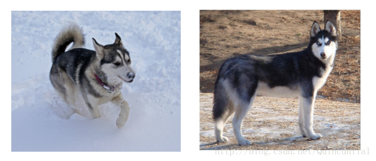
Bigger size typically means a larger number of parameters, which makes the enlarged network more prone to overfitting, especially if the number of labeled examples in the training set is limited. This is a major bottleneck as strongly labeled datasets are laborious and expensive to obtain, often requiring expert human raters to distinguish between various fine-grained visual categories such as those in ImageNet (even in the 1000-class ILSVRC subset) as shown in Figure 1.

Figure 1: Two distinct classes from the 1000 classes of the ILSVRC 2014 classification challenge. Domain knowledge is required to distinguish between these classes.

3. 动机和高层思考

提高深度神经网络性能最直接的方式是增加它们的尺寸。这不仅包括增加深度——网络层次的数目——也包括它的宽度：每一层的单元数目。这是一种训练更高质量模型容易且安全的方法，尤其是在可获得大量标注的训练数据的情况下。但是这个简单方案有两个主要的缺点。更大的尺寸通常意味着更多的参数，这会使增大的网络更容易过拟合，尤其是在训练集的标注样本有限的情况下。这是一个主要的瓶颈，因为要获得强标注数据集费时费力且代价昂贵，经常需要专家评委在各种细粒度的视觉类别进行区分，例如图1中显示的ImageNet中的类别（甚至是1000类ILSVRC的子集）。

图1: ILSVRC 2014分类挑战赛的1000类中两个不同的类别。区分这些类别需要领域知识。

The other drawback of uniformly increased network size is the dramatically increased use of computational resources. For example, in a deep vision network, if two convolutional layers are chained, any uniform increase in the number of their filters results in a quadratic increase of computation. If the added capacity is used inefficiently (for example, if most weights end up to be close to zero), then much of the computation is wasted. As the computational budget is always finite, an efficient distribution of computing resources is preferred to an indiscriminate increase of size, even when the main objective is to increase the quality of performance.

均匀增加网络尺寸的另一个缺点是计算资源使用的显著增加。例如，在一个深度视觉网络中，如果两个卷积层相连，它们的滤波器数目的任何均匀增加都会引起计算量平方式的增加。如果增加的能力使用时效率低下（例如，如果大多数权重结束时接近于0），那么会浪费大量的计算能力。由于计算预算总是有限的，计算资源的有效分布更偏向于尺寸无差别的增加，即使主要目标是增加性能的质量。

A fundamental way of solving both of these issues would be to introduce sparsity and replace the fully connected layers by the sparse ones, even inside the convolutions. Besides mimicking biological systems, this would also have the advantage of firmer theoretical underpinnings due to the groundbreaking work of Arora et al. [2]. Their main result states that if the probability distribution of the dataset is representable by a large, very sparse deep neural network, then the optimal network topology can be constructed layer after layer by analyzing the correlation statistics of the preceding layer activations and clustering neurons with highly correlated outputs. Although the strict mathematical proof requires very strong conditions, the fact that this statement resonates with the well known Hebbian principle —— neurons that fire together, wire together —— suggests that the underlying idea is applicable even under less strict conditions, in practice.

解决这两个问题的一个基本的方式就是引入稀疏性并将全连接层替换为稀疏的全连接层，甚至是卷积层。除了模仿生物系统之外，由于Arora等人[2]的开创性工作，这也具有更坚固的理论基础优势。他们的主要成果说明如果数据集的概率分布可以通过一个大型稀疏的深度神经网络表示，则最优的网络拓扑结构可以通过分析前一层激活的相关性统计和聚类高度相关的神经元来一层层的构建。虽然严格的数学证明需要在很强的条件下，但事实上这个声明与著名的赫布理论产生共鸣——神经元一起激发，一起连接——实践表明，基础概念甚至适用于不严格的条件下。

Unfortunately, today’s computing infrastructures are very inefficient when it comes to numerical calculation on non-uniform sparse data structures. Even if the number of arithmetic operations is reduced by 100×, the overhead of lookups and cache misses would dominate: switching to sparse matrices might not pay off. The gap is widened yet further by the use of steadily improving and highly tuned numerical libraries that allow for extremely fast dense matrix multiplication, exploiting the minute details of the underlying CPU or GPU hardware [16, 9]. Also, non-uniform sparse models require more sophisticated engineering and computing infrastructure. Most current vision oriented machine learning systems utilize sparsity in the spatial domain just by the virtue of employing convolutions. However, convolutions are implemented as collections of dense connections to the patches in the earlier layer. ConvNets have traditionally used random and sparse connection tables in the feature dimensions since [11] in order to break the symmetry and improve learning, yet the trend changed back to full connections with [9] in order to further optimize parallel computation. Current state-of-the-art architectures for computer vision have uniform structure. The large number of filters and greater batch size allows for the efficient use of dense computation.

遗憾的是，当碰到在非均匀的稀疏数据结构上进行数值计算时，现在的计算架构效率非常低下。即使算法运算的数量减少100倍，查询和缓存丢失上的开销仍占主导地位：切换到稀疏矩阵可能是不可行的。随着稳定提升和高度调整的数值库的应用，差距仍在进一步扩大，数值库要求极度快速密集的矩阵乘法，利用底层的CPU或GPU硬件[16, 9]的微小细节。非均匀的稀疏模型也要求更多的复杂工程和计算基础结构。目前大多数面向视觉的机器学习系统通过采用卷积的优点来利用空域的稀疏性。然而，卷积被实现为对上一层块的密集连接的集合。为了打破对称性，提高学习水平，从论文[11]开始，ConvNets习惯上在特征维度使用随机的稀疏连接表，然而为了进一步优化并行计算，论文[9]中趋向于变回全连接。目前最新的计算机视觉架构有统一的结构。更多的滤波器和更大的批大小要求密集计算的有效使用。

This raises the question of whether there is any hope for a next, intermediate step: an architecture that makes use of filter-level sparsity, as suggested by the theory, but exploits our current hardware by utilizing computations on dense matrices. The vast literature on sparse matrix computations (e.g. [3]) suggests that clustering sparse matrices into relatively dense submatrices tends to give competitive performance for sparse matrix multiplication. It does not seem far-fetched to think that similar methods would be utilized for the automated construction of non-uniform deep-learning architectures in the near future.

这提出了下一个中间步骤是否有希望的问题：一个架构能利用滤波器水平的稀疏性，正如理论所认为的那样，但能通过利用密集矩阵计算来利用我们目前的硬件。稀疏矩阵乘法的大量文献（例如[3]）认为对于稀疏矩阵乘法，将稀疏矩阵聚类为相对密集的子矩阵会有更佳的性能。在不久的将来会利用类似的方法来进行非均匀深度学习架构的自动构建，这样的想法似乎并不牵强。

The Inception architecture started out as a case study for assessing the hypothetical output of a sophisticated network topology construction algorithm that tries to approximate a sparse structure implied by [2] for vision networks and covering the hypothesized outcome by dense, readily available components. Despite being a highly speculative undertaking, modest gains were observed early on when compared with reference networks based on [12]. With a bit of tuning the gap widened and Inception proved to be especially useful in the context of localization and object detection as the base network for [6] and [5]. Interestingly, while most of the original architectural choices have been questioned and tested thoroughly in separation, they turned out to be close to optimal locally. One must be cautious though: although the Inception architecture has become a success for computer vision, it is still questionable whether this can be attributed to the guiding principles that have lead to its construction. Making sure of this would require a much more thorough analysis and verification.

Inception架构开始是作为案例研究，用于评估一个复杂网络拓扑构建算法的假设输出，该算法试图近似[2]中所示的视觉网络的稀疏结构，并通过密集的、容易获得的组件来覆盖假设结果。尽管是一个非常投机的事情，但与基于[12]的参考网络相比，早期可以观测到适度的收益。随着一点点调整加宽差距，作为[6]和[5]的基础网络，Inception被证明在定位上下文和目标检测中尤其有用。有趣的是，虽然大多数最初的架构选择已被质疑并分离开进行全面测试，但结果证明它们是局部最优的。然而必须谨慎：尽管Inception架构在计算机上领域取得成功，但这是否可以归因于构建其架构的指导原则仍是有疑问的。确保这一点将需要更彻底的分析和验证。

4. Architectural Details

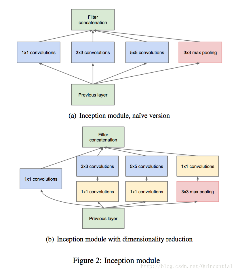
The main idea of the Inception architecture is to consider how an optimal local sparse structure of a convolutional vision network can be approximated and covered by readily available dense components. Note that assuming translation invariance means that our network will be built from convolutional building blocks. All we need is to find the optimal local construction and to repeat it spatially. Arora et al. [2] suggests a layer-by-layer construction where one should analyze the correlation statistics of the last layer and cluster them into groups of units with high correlation. These clusters form the units of the next layer and are connected to the units in the previous layer. We assume that each unit from an earlier layer corresponds to some region of the input image and these units are grouped into filter banks. In the lower layers (the ones close to the input) correlated units would concentrate in local regions. Thus, we would end up with a lot of clusters concentrated in a single region and they can be covered by a layer of 1×1 convolutions in the next layer, as suggested in [12]. However, one can also expect that there will be a smaller number of more spatially spread out clusters that can be covered by convolutions over larger patches, and there will be a decreasing number of patches over larger and larger regions. In order to avoid patch-alignment issues, current incarnations of the Inception architecture are restricted to filter sizes 1×1, 3×3 and 5×5; this decision was based more on convenience rather than necessity. It also means that the suggested architecture is a combination of all those layers with their output filter banks concatenated into a single output vector forming the input of the next stage. Additionally, since pooling operations have been essential for the success of current convolutional networks, it suggests that adding an alternative parallel pooling path in each such stage should have additional beneficial effect, too (see Figure 2(a)).

4. 架构细节

Inception架构的主要想法是考虑怎样近似卷积视觉网络的最优稀疏结构并用容易获得的密集组件进行覆盖。注意假设转换不变性，这意味着我们的网络将以卷积构建块为基础。我们所需要做的是找到最优的局部构造并在空间上重复它。Arora等人[2]提出了一个层次结构，其中应该分析最后一层的相关统计并将它们聚集成具有高相关性的单元组。这些聚类形成了下一层的单元并与前一层的单元连接。我们假设较早层的每个单元都对应输入层的某些区域，并且这些单元被分成滤波器组。在较低的层（接近输入的层）相关单元集中在局部区域。因此，如[12]所示，我们最终会有许多聚类集中在单个区域，它们可以通过下一层的1×1卷积层覆盖。然而也可以预期，将存在更小数目的在更大空间上扩展的聚类，其可以被更大块上的卷积覆盖，在越来越大的区域上块的数量将会下降。为了避免块校正的问题，目前Inception架构形式的滤波器的尺寸仅限于1×1、3×3、5×5，这个决定更多的是基于便易性而不是必要性。这也意味着提出的架构是所有这些层的组合，其输出滤波器组连接成单个输出向量形成了下一阶段的输入。另外，由于池化操作对于目前卷积网络的成功至关重要，因此建议在每个这样的阶段添加一个替代的并行池化路径应该也应该具有额外的有益效果（看图2(a)）。

As these “Inception modules” are stacked on top of each other, their output correlation statistics are bound to vary: as features of higher abstraction are captured by higher layers, their spatial concentration is expected to decrease. This suggests that the ratio of 3×3 and 5×5 convolutions should increase as we move to higher layers.

由于这些“Inception模块”在彼此的顶部堆叠，其输出相关统计必然有变化：由于较高层会捕获较高的抽象特征，其空间集中度预计会减少。这表明随着转移到更高层，3×3和5×5卷积的比例应该会增加。

One big problem with the above modules, at least in this naive form, is that even a modest number of 5×5 convolutions can be prohibitively expensive on top of a convolutional layer with a large number of filters. This problem becomes even more pronounced once pooling units are added to the mix: the number of output filters equals to the number of filters in the previous stage. The merging of output of the pooling layer with outputs of the convolutional layers would lead to an inevitable increase in the number of outputs from stage to stage. While this architecture might cover the optimal sparse structure, it would do it very inefficiently, leading to a computational blow up within a few stages.

上述模块的一个大问题是在具有大量滤波器的卷积层之上，即使适量的5×5卷积也可能是非常昂贵的，至少在这种朴素形式中有这个问题。一旦池化单元添加到混合中，这个问题甚至会变得更明显：输出滤波器的数量等于前一阶段滤波器的数量。池化层输出和卷积层输出的合并会导致这一阶段到下一阶段输出数量不可避免的增加。虽然这种架构可能会覆盖最优稀疏结构，但它会非常低效，导致在几个阶段内计算量爆炸。

This leads to the second idea of the Inception architecture: judiciously reducing dimension wherever the computational requirements would increase too much otherwise. This is based on the success of embeddings: even low dimensional embeddings might contain a lot of information about a relatively large image patch. However, embeddings represent information in a dense, compressed form and compressed information is harder to process. The representation should be kept sparse at most places (as required by the conditions of [2]) and compress the signals only whenever they have to be aggregated en masse. That is, 1×1 convolutions are used to compute reductions before the expensive 3×3 and 5×5 convolutions. Besides being used as reductions, they also include the use of rectified linear activation making them dual-purpose. The final result is depicted in Figure 2(b).

这导致了Inception架构的第二个想法：在计算要求会增加太多的地方，明智地减少维度。这是基于嵌入的成功：甚至低维嵌入可能包含大量关于较大图像块的信息。然而嵌入以密集、压缩形式表示信息并且压缩信息更难处理。这种表示应该在大多数地方保持稀疏（根据[2]中条件的要求】）并且仅在它们必须汇总时才压缩信号。也就是说，在昂贵的3×3和5×5卷积之前，1×1卷积用来计算降维。除了用来降维之外，它们也包括使用线性修正单元使其两用。最终的结果如图2(b)所示。

In general, an Inception network is a network consisting of modules of the above type stacked upon each other, with occasional max-pooling layers with stride 2 to halve the resolution of the grid. For technical reasons (memory efficiency during training), it seemed beneficial to start using Inception modules only at higher layers while keeping the lower layers in traditional convolutional fashion. This is not strictly necessary, simply reflecting some infrastructural inefficiencies in our current implementation.

通常，Inception网络是一个由上述类型的模块互相堆叠组成的网络，偶尔会有步长为2的最大池化层将网络分辨率减半。出于技术原因（训练过程中内存效率），只在更高层开始使用Inception模块而在更低层仍保持传统的卷积形式似乎是有益的。这不是绝对必要的，只是反映了我们目前实现中的一些基础结构效率低下。

A useful aspect of this architecture is that it allows for increasing the number of units at each stage significantly without an uncontrolled blow-up in computational complexity at later stages. This is achieved by the ubiquitous use of dimensionality reduction prior to expensive convolutions with larger patch sizes. Furthermore, the design follows the practical intuition that visual information should be processed at various scales and then aggregated so that the next stage can abstract features from the different scales simultaneously.

该架构的一个有用的方面是它允许显著增加每个阶段的单元数量，而不会在后面的阶段出现计算复杂度不受控制的爆炸。这是在尺寸较大的块进行昂贵的卷积之前通过普遍使用降维实现的。此外，设计遵循了实践直觉，即视觉信息应该在不同的尺度上处理然后聚合，为的是下一阶段可以从不同尺度同时抽象特征。

The improved use of computational resources allows for increasing both the width of each stage as well as the number of stages without getting into computational difficulties. One can utilize the Inception architecture to create slightly inferior, but computationally cheaper versions of it. We have found that all the available knobs and levers allow for a controlled balancing of computational resources resulting in networks that are 3—10× faster than similarly performing networks with non-Inception architecture, however this requires careful manual design at this point.

计算资源的改善使用允许增加每个阶段的宽度和阶段的数量，而不会陷入计算困境。可以利用Inception架构创建略差一些但计算成本更低的版本。我们发现所有可用的控制允许计算资源的受控平衡，导致网络比没有Inception结构的类似执行网络快3—10倍，但是在这一点上需要仔细的手动设计。

5. GoogLeNet

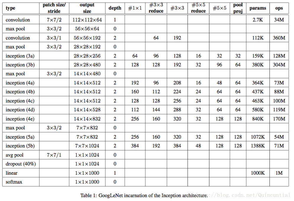
By the “GoogLeNet” name we refer to the particular incarnation of the Inception architecture used in our submission for the ILSVRC 2014 competition. We also used one deeper and wider Inception network with slightly superior quality, but adding it to the ensemble seemed to improve the results only marginally. We omit the details of that network, as empirical evidence suggests that the influence of the exact architectural parameters is relatively minor. Table 1 illustrates the most common instance of Inception used in the competition. This network (trained with different image patch sampling methods) was used for 6 out of the 7 models in our ensemble.

5. GoogLeNet

通过“GoogLeNet”这个名字，我们提到了在ILSVRC 2014竞赛的提交中使用的Inception架构的特例。我们也使用了一个稍微优质的更深更宽的Inception网络，但将其加入到组合中似乎只稍微提高了结果。我们忽略了该网络的细节，因为经验证据表明确切架构的参数影响相对较小。表1说明了竞赛中使用的最常见的Inception实例。这个网络（用不同的图像块采样方法训练的）使用了我们组合中7个模型中的6个。

All the convolutions, including those inside the Inception modules, use rectified linear activation. The size of the receptive field in our network is 224×224 in the RGB color space with zero mean. “#3×3 reduce” and “#5×5 reduce” stands for the number of 1×1 filters in the reduction layer used before the 3×3 and 5×5 convolutions. One can see the number of 1×1 filters in the projection layer after the built-in max-pooling in the pool proj column. All these reduction/projection layers use rectified linear activation as well.

所有的卷积都使用了修正线性激活，包括Inception模块内部的卷积。在我们的网络中感受野是在均值为0的RGB颜色空间中，大小是224×224。“#3×3 reduce”和“#5×5 reduce”表示在3×3和5×5卷积之前，降维层使用的1×1滤波器的数量。在pool proj列可以看到内置的最大池化之后，投影层中1×1滤波器的数量。所有的这些降维/投影层也都使用了线性修正激活。

The network was designed with computational efficiency and practicality in mind, so that inference can be run on individual devices including even those with limited computational resources, especially with low-memory footprint.The network is 22 layers deep when counting only layers with parameters (or 27 layers if we also count pooling). The overall number of layers (independent building blocks) used for the construction of the network is about 100. The exact number depends on how layers are counted by the machine learning infrastructure. The use of average pooling before the classifier is based on [12], although our implementation has an additional linear layer. The linear layer enables us to easily adapt our networks to other label sets, however it is used mostly for convenience and we do not expect it to have a major effect. We found that a move from fully connected layers to average pooling improved the top-1 accuracy by about 0.6%, however the use of dropout remained essential even after removing the fully connected layers.

网络的设计考虑了计算效率和实用性，因此推断可以单独的设备上运行，甚至包括那些计算资源有限的设备，尤其是低内存占用的设备。当只计算有参数的层时，网络有22层（如果我们也计算池化层是27层）。构建网络的全部层（独立构建块）的数目大约是100。确切的数量取决于机器学习基础设施对层的计算方式。分类器之前的平均池化是基于[12]的，尽管我们的实现有一个额外的线性层。线性层使我们的网络能很容易地适应其它的标签集，但它主要是为了方便使用，我们不期望它有重大的影响。我们发现从全连接层变为平均池化，提高了大约top-1 %0.6的准确率，然而即使在移除了全连接层之后，丢失的使用还是必不可少的。

Given relatively large depth of the network, the ability to propagate gradients back through all the layers in an effective manner was a concern. The strong performance of shallower networks on this task suggests that the features produced by the layers in the middle of the network should be very discriminative. By adding auxiliary classifiers connected to these intermediate layers, discrimination in the lower stages in the classifier was expected. This was thought to combat the vanishing gradient problem while providing regularization. These classifiers take the form of smaller convolutional networks put on top of the output of the Inception (4a) and (4d) modules. During training, their loss gets added to the total loss of the network with a discount weight (the losses of the auxiliary classifiers were weighted by 0.3). At inference time, these auxiliary networks are discarded. Later control experiments have shown that the effect of the auxiliary networks is relatively minor (around 0.5%) and that it required only one of them to achieve the same effect.

给定深度相对较大的网络，有效传播梯度反向通过所有层的能力是一个问题。在这个任务上，更浅网络的强大性能表明网络中部层产生的特征应该是非常有识别力的。通过将辅助分类器添加到这些中间层，可以期望较低阶段分类器的判别力。这被认为是在提供正则化的同时克服梯度消失问题。这些分类器采用较小卷积网络的形式，放置在Inception (4a)和Inception (4b)模块的输出之上。在训练期间，它们的损失以折扣权重（辅助分类器损失的权重是0.3）加到网络的整个损失上。在推断时，这些辅助网络被丢弃。后面的控制实验表明辅助网络的影响相对较小（约0.5），只需要其中一个就能取得同样的效果。

The exact structure of the extra network on the side, including the auxiliary classifier, is as follows:

• An average pooling layer with 5×5 filter size and stride 3, resulting in an 4×4×512 output for the (4a), and 4×4×528 for the (4d) stage.
• A 1×1 convolution with 128 filters for dimension reduction and rectified linear activation.
• A fully connected layer with 1024 units and rectified linear activation.
• A dropout layer with 70% ratio of dropped outputs.
• A linear layer with softmax loss as the classifier (predicting the same 1000 classes as the main classifier, but removed at inference time).

A schematic view of the resulting network is depicted in Figure 3.

Figure 3: GoogLeNet network with all the bells and whistles.

包括辅助分类器在内的附加网络的具体结构如下：

• 一个滤波器大小5×5，步长为3的平均池化层，导致(4a)阶段的输出为4×4×512，(4d)的输出为4×4×528。
• 具有128个滤波器的1×1卷积，用于降维和修正线性激活。
• 一个全连接层，具有1024个单元和修正线性激活。
• 丢弃70%输出的丢弃层。
• 使用带有softmax损失的线性层作为分类器（作为主分类器预测同样的1000类，但在推断时移除）。

最终的网络模型图如图3所示。

图3：含有的所有结构的GoogLeNet网络。

6. Training Methodology

GoogLeNet networks were trained using the DistBelief [4] distributed machine learning system using modest amount of model and data-parallelism. Although we used a CPU based implementation only, a rough estimate suggests that the GoogLeNet network could be trained to convergence using few high-end GPUs within a week, the main limitation being the memory usage. Our training used asynchronous stochastic gradient descent with 0.9 momentum [17], fixed learning rate schedule (decreasing the learning rate by 4% every 8 epochs). Polyak averaging [13] was used to create the final model used at inference time.

6. 训练方法

GoogLeNet网络使用DistBelief[4]分布式机器学习系统进行训练，该系统使用适量的模型和数据并行。尽管我们仅使用一个基于CPU的实现，但粗略的估计表明GoogLeNet网络可以用更少的高端GPU在一周之内训练到收敛，主要的限制是内存使用。我们的训练使用异步随机梯度下降，动量参数为0.9[17]，固定的学习率计划（每8次遍历下降学习率4%）。Polyak平均[13]在推断时用来创建最终的模型。

Image sampling methods have changed substantially over the months leading to the competition, and already converged models were trained on with other options, sometimes in conjunction with changed hyperparameters, such as dropout and the learning rate. Therefore, it is hard to give a definitive guidance to the most effective single way to train these networks. To complicate matters further, some of the models were mainly trained on smaller relative crops, others on larger ones, inspired by [8]. Still, one prescription that was verified to work very well after the competition, includes sampling of various sized patches of the image whose size is distributed evenly between 8% and 100% of the image area with aspect ratio constrained to the interval $[\frac {3} {4}, \frac {4} {3}]$. Also, we found that the photometric distortions of Andrew Howard [8] were useful to combat overfitting to the imaging conditions of training data.

图像采样方法在过去几个月的竞赛中发生了重大变化，并且已收敛的模型在其他选项上进行了训练，有时还结合着超参数的改变，例如丢弃和学习率。因此，很难对训练这些网络的最有效的单一方式给出明确指导。让事情更复杂的是，受[8]的启发，一些模型主要是在相对较小的裁剪图像进行训练，其它模型主要是在相对较大的裁剪图像上进行训练。然而，一个经过验证的方案在竞赛后工作地很好，包括各种尺寸的图像块的采样，它的尺寸均匀分布在图像区域的8%——100%之间，方向角限制为$[\frac {3} {4}, \frac {4} {3}]$之间。另外，我们发现Andrew Howard[8]的光度扭曲对于克服训练数据成像条件的过拟合是有用的。

7. ILSVRC 2014 Classification Challenge Setup and Results

The ILSVRC 2014 classification challenge involves the task of classifying the image into one of 1000 leaf-node categories in the Imagenet hierarchy. There are about 1.2 million images for training, 50,000 for validation and 100,000 images for testing. Each image is associated with one ground truth category, and performance is measured based on the highest scoring classifier predictions. Two numbers are usually reported: the top-1 accuracy rate, which compares the ground truth against the first predicted class, and the top-5 error rate, which compares the ground truth against the first 5 predicted classes: an image is deemed correctly classified if the ground truth is among the top-5, regardless of its rank in them. The challenge uses the top-5 error rate for ranking purposes.

7. ILSVRC 2014分类挑战赛设置和结果

ILSVRC 2014分类挑战赛包括将图像分类到ImageNet层级中1000个叶子结点类别的任务。训练图像大约有120万张，验证图像有5万张，测试图像有10万张。每一张图像与一个实际类别相关联，性能度量基于分类器预测的最高分。通常报告两个数字：top-1准确率，比较实际类别和第一个预测类别，top-5错误率，比较实际类别与前5个预测类别：如果图像实际类别在top-5中，则认为图像分类正确，不管它在top-5中的排名。挑战赛使用top-5错误率来进行排名。

We participated in the challenge with no external data used for training. In addition to the training techniques aforementioned in this paper, we adopted a set of techniques during testing to obtain a higher performance, which we describe next.

1. We independently trained 7 versions of the same GoogLeNet model (including one wider version), and performed ensemble prediction with them. These models were trained with the same initialization (even with the same initial weights, due to an oversight) and learning rate policies. They differed only in sampling methodologies and the randomized input image order.
2. During testing, we adopted a more aggressive cropping approach than that of Krizhevsky et al. [9]. Specifically, we resized the image to 4 scales where the shorter dimension (height or width) is 256, 288, 320 and 352 respectively, take the left, center and right square of these resized images (in the case of portrait images, we take the top, center and bottom squares). For each square, we then take the 4 corners and the center 224×224 crop as well as the square resized to 224×224, and their mirrored versions. This leads to 4×3×6×2 = 144 crops per image. A similar approach was used by Andrew Howard [8] in the previous year’s entry, which we empirically verified to perform slightly worse than the proposed scheme. We note that such aggressive cropping may not be necessary in real applications, as the benefit of more crops becomes marginal after a reasonable number of crops are present (as we will show later on).
3. The softmax probabilities are averaged over multiple crops and over all the individual classifiers to obtain the final prediction. In our experiments we analyzed alternative approaches on the validation data, such as max pooling over crops and averaging over classifiers, but they lead to inferior performance than the simple averaging.

我们参加竞赛时没有使用外部数据来训练。除了本文中前面提到的训练技术之外，我们在获得更高性能的测试中采用了一系列技巧，描述如下。

1. 我们独立训练了7个版本的相同的GoogLeNet模型（包括一个更广泛的版本），并用它们进行了整体预测。这些模型的训练具有相同的初始化（甚至具有相同的初始权重，由于监督）和学习率策略。它们仅在采样方法和随机输入图像顺序方面不同。
2. 在测试中，我们采用比Krizhevsky等人[9]更积极的裁剪方法。具体来说，我们将图像归一化为四个尺度，其中较短维度（高度或宽度）分别为256，288，320和352，取这些归一化的图像的左，中，右方块（在肖像图片中，我们采用顶部，中心和底部方块）。对于每个方块，我们将采用4个角以及中心224×224裁剪图像以及方块尺寸归一化为224×224，以及它们的镜像版本。这导致每张图像会得到4×3×6×2 = 144的裁剪图像。前一年的输入中，Andrew Howard[8]采用了类似的方法，经过我们实证验证，其方法略差于我们提出的方案。我们注意到，在实际应用中，这种积极裁剪可能是不必要的，因为存在合理数量的裁剪图像后，更多裁剪图像的好处会变得很微小（正如我们后面展示的那样）。
3. softmax概率在多个裁剪图像上和所有单个分类器上进行平均，然后获得最终预测。在我们的实验中，我们分析了验证数据的替代方法，例如裁剪图像上的最大池化和分类器的平均，但是它们比简单平均的性能略逊。

In the remainder of this paper, we analyze the multiple factors that contribute to the overall performance of the final submission.

在本文的其余部分，我们分析了有助于最终提交整体性能的多个因素。

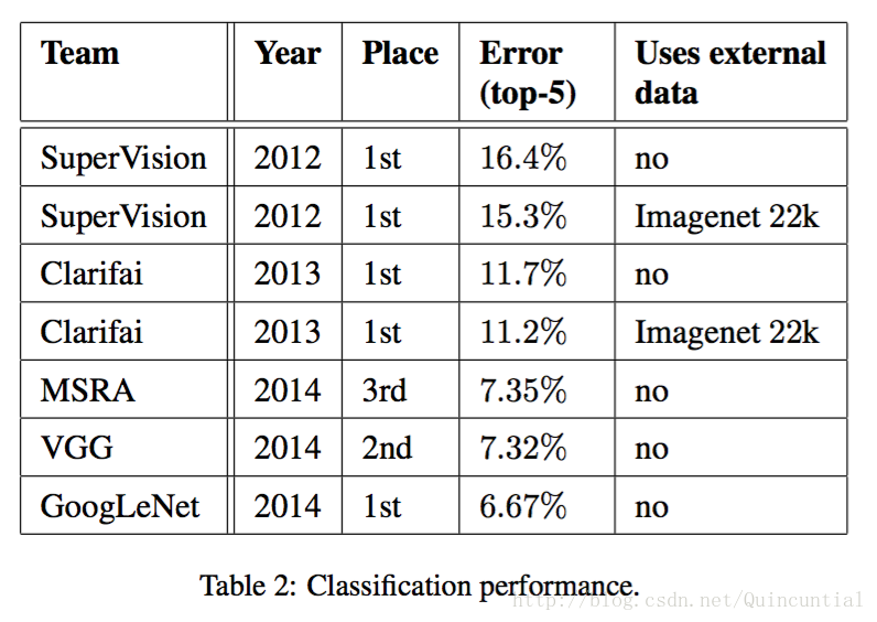
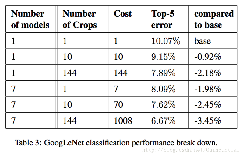
Our final submission to the challenge obtains a top-5 error of 6.67% on both the validation and testing data, ranking the first among other participants. This is a 56.5% relative reduction compared to the SuperVision approach in 2012, and about 40% relative reduction compared to the previous year’s best approach (Clarifai), both of which used external data for training the classifiers. Table 2 shows the statistics of some of the top-performing approaches over the past 3 years.

竞赛中我们的最终提交在验证集和测试集上得到了top-5 6.67%的错误率，在其它的参与者中排名第一。与2012年的SuperVision方法相比相对减少了56.5%，与前一年的最佳方法（Clarifai）相比相对减少了约40%，这两种方法都使用了外部数据训练分类器。表2显示了过去三年中一些表现最好的方法的统计。

We also analyze and report the performance of multiple testing choices, by varying the number of models and the number of crops used when predicting an image in Table 3. When we use one model, we chose the one with the lowest top-1 error rate on the validation data. All numbers are reported on the validation dataset in order to not overfit to the testing data statistics.

我们也分析报告了多种测试选择的性能，当预测图像时通过改变表3中使用的模型数目和裁剪图像数目。

8. ILSVRC 2014 Detection Challenge Setup and Results

The ILSVRC detection task is to produce bounding boxes around objects in images among 200 possible classes. Detected objects count as correct if they match the class of the groundtruth and their bounding boxes overlap by at least 50% (using the Jaccard index). Extraneous detections count as false positives and are penalized. Contrary to the classification task, each image may contain many objects or none, and their scale may vary. Results are reported using the mean average precision (mAP). The approach taken by GoogLeNet for detection is similar to the R-CNN by [6], but is augmented with the Inception model as the region classifier. Additionally, the region proposal step is improved by combining the selective search [20] approach with multi-box [5] predictions for higher object bounding box recall. In order to reduce the number of false positives, the superpixel size was increased by 2×. This halves the proposals coming from the selective search algorithm. We added back 200 region proposals coming from multi-box [5] resulting, in total, in about 60% of the proposals used by [6], while increasing the coverage from 92% to 93%. The overall effect of cutting the number of proposals with increased coverage is a 1% improvement of the mean average precision for the single model case. Finally, we use an ensemble of 6 GoogLeNets when classifying each region. This leads to an increase in accuracy from 40% to 43.9%. Note that contrary to R-CNN, we did not use bounding box regression due to lack of time.

8. ILSVRC 2014检测挑战赛设置和结果

ILSVRC检测任务是为了在200个可能的类别中生成图像中目标的边界框。如果检测到的对象匹配的它们实际类别并且它们的边界框重叠至少50%（使用Jaccard索引），则将检测到的对象记为正确。无关的检测记为假阳性且被惩罚。与分类任务相反，每张图像可能包含多个对象或没有对象，并且它们的尺度可能是变化的。报告的结果使用平均精度均值（mAP）。GoogLeNet检测采用的方法类似于R-CNN[6]，但用Inception模块作为区域分类器进行了增强。此外，为了更高的目标边界框召回率，通过选择搜索[20]方法和多箱[5]预测相结合改进了区域生成步骤。为了减少假阳性的数量，超分辨率的尺寸增加了2倍。这将选择搜索算法的区域生成减少了一半。我们总共补充了200个来自多盒结果的区域生成，大约60%的区域生成用于[6]，同时将覆盖率从92%提高到93%。减少区域生成的数量，增加覆盖率的整体影响是对于单个模型的情况平均精度均值增加了1%。最后，等分类单个区域时，我们使用了6个GoogLeNets的组合。这导致准确率从40%提高到43.9%。注意，与R-CNN相反，由于缺少时间我们没有使用边界框回归。

We first report the top detection results and show the progress since the first edition of the detection task. Compared to the 2013 result, the accuracy has almost doubled. The top performing teams all use convolutional networks. We report the official scores in Table 4 and common strategies for each team: the use of external data, ensemble models or contextual models. The external data is typically the ILSVRC12 classification data for pre-training a model that is later refined on the detection data. Some teams also mention the use of the localization data. Since a good portion of the localization task bounding boxes are not included in the detection dataset, one can pre-train a general bounding box regressor with this data the same way classification is used for pre-training. The GoogLeNet entry did not use the localization data for pretraining.

我们首先报告了最好检测结果，并显示了从第一版检测任务以来的进展。与2013年的结果相比，准确率几乎翻了一倍。所有表现最好的团队都使用了卷积网络。我们在表4中报告了官方的分数和每个队伍的常见策略：使用外部数据、集成模型或上下文模型。外部数据通常是ILSVRC12的分类数据，用来预训练模型，后面在检测数据集上进行改善。一些团队也提到使用定位数据。由于定位任务的边界框很大一部分不在检测数据集中，所以可以用该数据预训练一般的边界框回归器，这与分类预训练的方式相同。GoogLeNet输入没有使用定位数据进行预训练。

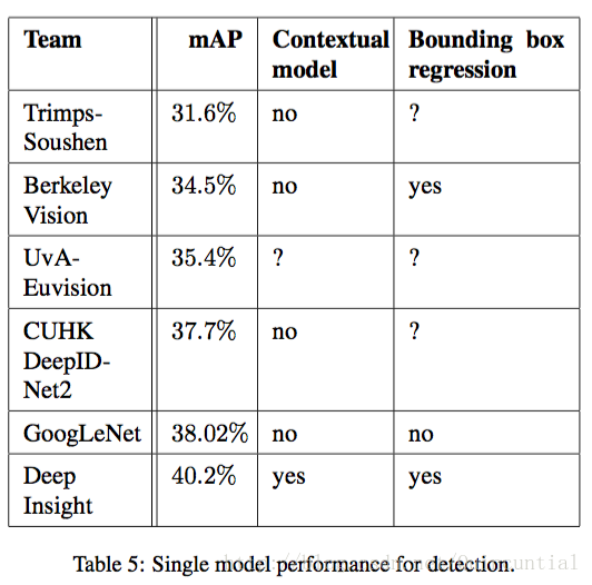
In Table 5, we compare results using a single model only. The top performing model is by Deep Insight and surprisingly only improves by 0.3 points with an ensemble of 3 models while the GoogLeNet obtains significantly stronger results with the ensemble.

在表5中，我们仅比较了单个模型的结果。最好性能模型是Deep Insight的，令人惊讶的是3个模型的集合仅提高了0.3个点，而GoogLeNet在模型集成时明显获得了更好的结果。

9. Conclusions

Our results yield a solid evidence that approximating the expected optimal sparse structure by readily available dense building blocks is a viable method for improving neural networks for computer vision. The main advantage of this method is a significant quality gain at a modest increase of computational requirements compared to shallower and narrower architectures.

9. 总结

我们的结果取得了可靠的证据，即通过易获得的密集构造块来近似期望的最优稀疏结果是改善计算机视觉神经网络的一种可行方法。相比于较浅且较窄的架构，这个方法的主要优势是在计算需求适度增加的情况下有显著的质量收益。

Our object detection work was competitive despite not utilizing context nor performing bounding box regression, suggesting yet further evidence of the strengths of the Inception architecture.

我们的目标检测工作虽然没有利用上下文，也没有执行边界框回归，但仍然具有竞争力，这进一步显示了Inception架构优势的证据。

For both classification and detection, it is expected that similar quality of result can be achieved by much more expensive non-Inception-type networks of similar depth and width. Still, our approach yields solid evidence that moving to sparser architectures is feasible and useful idea in general. This suggest future work towards creating sparser and more refined structures in automated ways on the basis of [2], as well as on applying the insights of the Inception architecture to other domains.

对于分类和检测，预期通过更昂贵的类似深度和宽度的非Inception类型网络可以实现类似质量的结果。 然而，我们的方法取得了可靠的证据，即转向更稀疏的结构一般来说是可行有用的想法。这表明未来的工作将在[2]的基础上以自动化方式创建更稀疏更精细的结构，以及将Inception架构的思考应用到其他领域。

References

[1] Know your meme: We need to go deeper. http://knowyourmeme.com/memes/we-need-to-go-deeper. Accessed: 2014-09-15.

[2] S. Arora, A. Bhaskara, R. Ge, and T. Ma. Provable bounds for learning some deep representations. CoRR, abs/1310.6343, 2013.

[3] U. V. C ?atalyu ?rek, C. Aykanat, and B. Uc ?ar. On two-dimensional sparse matrix partitioning: Models, methods, and a recipe. SIAM J. Sci. Comput., 32(2):656–683, Feb. 2010.

[4] J. Dean, G. Corrado, R. Monga, K. Chen, M. Devin, M. Mao, M. Ranzato, A. Senior, P. Tucker, K. Yang, Q. V. Le, and A. Y. Ng. Large scale distributed deep networks. In P. Bartlett, F. Pereira, C. Burges, L. Bottou, and K. Weinberger, editors, NIPS, pages 1232–1240. 2012.

[5] D. Erhan, C. Szegedy, A. Toshev, and D. Anguelov. Scalable object detection using deep neural networks. In CVPR, 2014.

[6] R. B. Girshick, J. Donahue, T. Darrell, and J. Malik. Rich feature hierarchies for accurate object detection and semantic segmentation. In Computer Vision and Pattern Recognition, 2014. CVPR 2014. IEEE Conference on, 2014.

[7] G. E. Hinton, N. Srivastava, A. Krizhevsky, I. Sutskever, and R. Salakhutdinov. Improving neural networks by preventing co-adaptation of feature detectors. CoRR, abs/1207.0580, 2012.

[8] A. G. Howard. Some improvements on deep convolutional neural network based image classification. CoRR, abs/1312.5402, 2013.

[9] A. Krizhevsky, I. Sutskever, and G. Hinton. Imagenet classification with deep convolutional neural networks. In Advances in Neural Information Processing Systems 25, pages 1106–1114, 2012.

[10] Y. LeCun, B. Boser, J. S. Denker, D. Henderson, R. E. Howard, W. Hubbard, and L. D. Jackel. Backpropagation applied to handwritten zip code recognition. Neural Comput., 1(4):541–551, Dec. 1989.

[11] Y. LeCun, L. Bottou, Y. Bengio, and P. Haffner. Gradient-based learning applied to document recognition. Proceedings of the IEEE, 86(11):2278–2324, 1998.

[12] M. Lin, Q. Chen, and S. Yan. Network in network. CoRR, abs/1312.4400, 2013.

[13] B. T. Polyak and A. B. Juditsky. Acceleration of stochastic approximation by averaging. SIAM J. Control Optim., 30(4):838–855, July 1992.

[14] P. Sermanet, D. Eigen, X. Zhang, M. Mathieu, R. Fergus, and Y. LeCun. Overfeat: Integrated recognition, localization and detection using convolutional networks. CoRR, abs/1312.6229, 2013.

[15] T. Serre, L. Wolf, S. M. Bileschi, M. Riesenhuber, and T. Poggio. Robust object recognition with cortex-like mechanisms. IEEE Trans. Pattern Anal. Mach. Intell., 29(3):411–426, 2007.

[16] F. Song and J. Dongarra. Scaling up matrix computations on shared-memory manycore systems with 1000 cpu cores. In Proceedings of the 28th ACM Interna- tional Conference on Supercomputing, ICS ’14, pages 333–342, New York, NY, USA, 2014. ACM.

[17] I. Sutskever, J. Martens, G. E. Dahl, and G. E. Hinton. On the importance of initialization and momentum in deep learning. In ICML, volume 28 of JMLR Proceed- ings, pages 1139–1147. JMLR.org, 2013.

[18] C.Szegedy,A.Toshev,andD.Erhan.Deep neural networks for object detection. In C. J. C. Burges, L. Bottou, Z. Ghahramani, and K. Q. Weinberger, editors, NIPS, pages 2553–2561, 2013.

[19] A. Toshev and C. Szegedy. Deeppose: Human pose estimation via deep neural networks. CoRR, abs/1312.4659, 2013.

[20] K. E. A. van de Sande, J. R. R. Uijlings, T. Gevers, and A. W. M. Smeulders. Segmentation as selective search for object recognition. In Proceedings of the 2011 International Conference on Computer Vision, ICCV ’11, pages 1879–1886, Washington, DC, USA, 2011. IEEE Computer Society.

[21] M. D. Zeiler and R. Fergus. Visualizing and understanding convolutional networks. In D. J. Fleet, T. Pajdla, B. Schiele, and T. Tuytelaars, editors, ECCV, volume 8689 of Lecture Notes in Computer Science, pages 818–833. Springer, 2014.