Matlab兑现线性回归和逻辑回归: Linear Regression & Logistic Regression_GIS

Matlab实现线性回归和逻辑回归: Linear Regression & Logistic Regression

本文为Maching Learning 栏目补充内容，为上几章中所提到单参数线性回归、多参数线性回归和逻辑回归的总结版。旨在帮助大家更好地理解回归，所以我在Matlab中分别对他们予以实现，在本文中由易到难地逐个介绍。

本讲内容：

Matlab 实现各种回归函数

=========================

基本模型

Y=θ₀+θ₁X₁型---线性回归（直线拟合）

解决过拟合问题---Regularization

Y=1/(1+e^X)型---逻辑回归（sigmod 函数拟合）

=========================

第一部分：基本模型

在解决拟合问题的解决之前，我们首先回忆一下线性回归和逻辑回归的基本模型。

设待拟合参数 θ_n*1 和输入参数[ x_m*n, y_m*1] 。

对于各类拟合我们都要根据梯度下降的算法，给出两部分：

① cost function（指出真实值y与拟合值h<hypothesis>之间的距离）：给出cost function 的表达式，每次迭代保证cost function的量减小；给出梯度gradient，即cost function对每一个参数θ的求导结果。

function [ jVal,gradient ] = costFunction ( theta )

② Gradient_descent（主函数）：用来运行梯度下降算法，调用上面的cost function进行不断迭代，直到最大迭代次数达到给定标准或者cost function返回值不再减小。

function [optTheta,functionVal,exitFlag]=Gradient_descent( )

线性回归：拟合方程为h_θ(x)=θ₀x₀+θ₁x₁+…+θ_nx_n，当然也可以有x_n的幂次方作为线性回归项（如），这与普通意义上的线性不同，而是类似多项式的概念。

其cost function 为：

逻辑回归：拟合方程为h_θ(x)=1/(1+e^(θ^Tx))，其cost function 为：

cost function对各θj的求导请自行求取，看第三章最后一图，或者参见后文代码。

_{后面，我们分别对几个模型方程进行拟合，给出代码，并用matlab中的fit函数进行验证。}

第二部分：Y=θ₀+θ₁X₁型---线性回归（直线拟合）

在Matlab 线性拟合 & 非线性拟合中我们已经讲过如何用matlab自带函数fit进行直线和曲线的拟合，非常实用。而这里我们是进行ML课程的学习，因此研究如何利用前面讲到的梯度下降法（gradient descent）进行拟合。

cost function：

function [ jVal,gradient ] = costFunction2( theta )%COSTFUNCTION2 Summary of this function goes here%   linear regression -> y=theta0 + theta1*x%   parameter: x:m*n  theta:n*1   y:m*1   (m=4,n=1)%   %Datax=[1;2;3;4];y=[1.1;2.2;2.7;3.8];m=size(x,1);hypothesis = h_func(x,theta);delta = hypothesis - y;jVal=sum(delta.^2);gradient(1)=sum(delta)/m;gradient(2)=sum(delta.*x)/m;end

其中，h_func是hypothesis的结果：

function [res] = h_func(inputx,theta)%H_FUNC Summary of this function goes here%   Detailed explanation goes here%cost function 2res= theta(1)+theta(2)*inputx;function [res] = h_func(inputx,theta)end

Gradient_descent：

function [optTheta,functionVal,exitFlag]=Gradient_descent( )%GRADIENT_DESCENT Summary of this function goes here%   Detailed explanation goes here  options = optimset('GradObj','on','MaxIter',100);  initialTheta = zeros(2,1);  [optTheta,functionVal,exitFlag] = fminunc(@costFunction2,initialTheta,options);end

result：

>> [optTheta,functionVal,exitFlag] = Gradient_descent()Local minimum found.Optimization completed because the size of the gradient is less thanthe default value of the function tolerance.<stopping criteria details>optTheta =    0.3000    0.8600functionVal =    0.0720exitFlag =     1

即得y=0.3+0.86x;

验证：

function [ parameter ] = checkcostfunc(  )%CHECKC2 Summary of this function goes here%   check if the cost function works well%   check with the matlab fit function as standard%check cost function 2x=[1;2;3;4];y=[1.1;2.2;2.7;3.8];EXPR= {'x','1'};p=fittype(EXPR);parameter=fit(x,y,p);end

运行结果：

>> checkcostfunc()ans =      Linear model:     ans(x) = a*x + b     Coefficients (with 95% confidence bounds):       a =        0.86  (0.4949, 1.225)       b =         0.3  (-0.6998, 1.3)

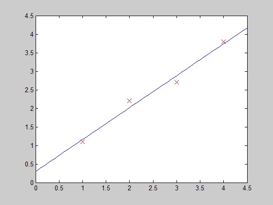
和我们的结果一样。下面画图：

function PlotFunc( xstart,xend )%PLOTFUNC Summary of this function goes here%   draw original data and the fitted %===================cost function 2====linear regression%original datax1=[1;2;3;4];y1=[1.1;2.2;2.7;3.8];%plot(x1,y1,'ro-','MarkerSize',10);plot(x1,y1,'rx','MarkerSize',10);hold on;%fitted line - 拟合曲线x_co=xstart:0.1:xend;y_co=0.3+0.86*x_co;%plot(x_co,y_co,'g');plot(x_co,y_co);hold off;end

第三部分：解决过拟合问题---Regularization

过拟合问题解决方法我们已在第三章中讲过，利用Regularization的方法就是在cost function中加入关于θ的项，使得部分θ的值偏小，从而达到fit效果。

例如定义costfunction J(θ)： jVal=(theta(1)-5)^2+(theta(2)-5)^2;

在每次迭代中，按照gradient descent的方法更新参数θ：θ(i)-=gradient(i),其中gradient(i)是J(θ)对θi求导的函数式，在此例中就有gradient(1)=2*(theta(1)-5), gradient(2)=2*(theta(2)-5)。

函数costFunction, 定义jVal=J(θ)和对两个θ的gradient：

function [ jVal,gradient ] = costFunction( theta )%COSTFUNCTION Summary of this function goes here%   Detailed explanation goes herejVal= (theta(1)-5)^2+(theta(2)-5)^2;gradient = zeros(2,1);%code to compute derivative to thetagradient(1) = 2 * (theta(1)-5);gradient(2) = 2 * (theta(2)-5);end

Gradient_descent，进行参数优化

function [optTheta,functionVal,exitFlag]=Gradient_descent( )%GRADIENT_DESCENT Summary of this function goes here%   Detailed explanation goes here options = optimset('GradObj','on','MaxIter',100); initialTheta = zeros(2,1) [optTheta,functionVal,exitFlag] = fminunc(@costFunction,initialTheta,options);  end

matlab主窗口中调用，得到优化厚的参数(θ1,θ2)=(5,5)

 [optTheta,functionVal,exitFlag] = Gradient_descent()initialTheta =     0     0Local minimum found.Optimization completed because the size of the gradient is less thanthe default value of the function tolerance.<stopping criteria details>optTheta =     5     5functionVal =     0exitFlag =     1

第四部分：Y=1/(1+e^X)型---逻辑回归（sigmod 函数拟合）

hypothesis function:

function [res] = h_func(inputx,theta)%cost function 3tmp=theta(1)+theta(2)*inputx;%m*1res=1./(1+exp(-tmp));%m*1end

cost function:

function [ jVal,gradient ] = costFunction3( theta )%COSTFUNCTION3 Summary of this function goes here%   Logistic Regressionx=[-3;      -2;     -1;     0;      1;      2;     3];y=[0.01;    0.05;   0.3;    0.45;   0.8;    1.1;    0.99];m=size(x,1);%hypothesis  datahypothesis = h_func(x,theta);%jVal-cost function  &  gradient updatingjVal=-sum(log(hypothesis+0.01).*y + (1-y).*log(1-hypothesis+0.01))/m;gradient(1)=sum(hypothesis-y)/m;   %reflect to theta1gradient(2)=sum((hypothesis-y).*x)/m;    %reflect to theta 2end

Gradient_descent:

function [optTheta,functionVal,exitFlag]=Gradient_descent( ) options = optimset('GradObj','on','MaxIter',100); initialTheta = [0;0]; [optTheta,functionVal,exitFlag] = fminunc(@costFunction3,initialTheta,options);end

运行结果：

 [optTheta,functionVal,exitFlag] = Gradient_descent()Local minimum found.Optimization completed because the size of the gradient is less thanthe default value of the function tolerance.<stopping criteria details>optTheta =    0.3526    1.7573functionVal =    0.2498exitFlag =     1

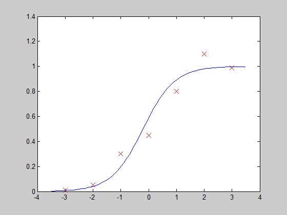
画图验证：

function PlotFunc( xstart,xend )%PLOTFUNC Summary of this function goes here%   draw original data and the fitted %===================cost function 3=====logistic regression%original datax=[-3;      -2;     -1;     0;      1;      2;     3];y=[0.01;    0.05;   0.3;    0.45;   0.8;    1.1;    0.99];plot(x,y,'rx','MarkerSize',10);hold on%fitted linex_co=xstart:0.1:xend;theta = [0.3526,1.7573];y_co=h_func(x_co,theta);plot(x_co,y_co);hold offend

==============================

Reference:

1. http://blog.csdn.net/abcjennifer/article/details/7691571

2.http://blog.csdn.net/abcjennifer/article/details/7700772

3.http://blog.csdn.net/abcjennifer/article/details/7716281

4.http://blog.csdn.net/abcjennifer/article/details/7684836